# A tibble: 25,534 × 34
Longitude Latitude UserID Genus Family DBH Inventory_Date Species
<dbl> <dbl> <dbl> <chr> <chr> <dbl> <dttm> <chr>
1 -123. 45.6 1 Pseudotsu… Pinac… 37.4 2017-05-09 00:00:00 PSME
2 -123. 45.6 2 Pseudotsu… Pinac… 32.5 2017-05-09 00:00:00 PSME
3 -123. 45.6 3 Crataegus Rosac… 9.7 2017-05-09 00:00:00 CRLA
4 -123. 45.6 4 Quercus Fagac… 10.3 2017-05-09 00:00:00 QURU
5 -123. 45.6 5 Pseudotsu… Pinac… 33.2 2017-05-09 00:00:00 PSME
6 -123. 45.6 6 Pseudotsu… Pinac… 32.1 2017-05-09 00:00:00 PSME
7 -123. 45.6 7 Pseudotsu… Pinac… 28.4 2017-05-09 00:00:00 PSME
8 -123. 45.6 8 Pseudotsu… Pinac… 27.2 2017-05-09 00:00:00 PSME
9 -123. 45.6 9 Pseudotsu… Pinac… 35.2 2017-05-09 00:00:00 PSME
10 -123. 45.6 10 Pseudotsu… Pinac… 32.4 2017-05-09 00:00:00 PSME
# ℹ 25,524 more rows
# ℹ 26 more variables: Common_Name <chr>, Condition <chr>, Tree_Height <dbl>,
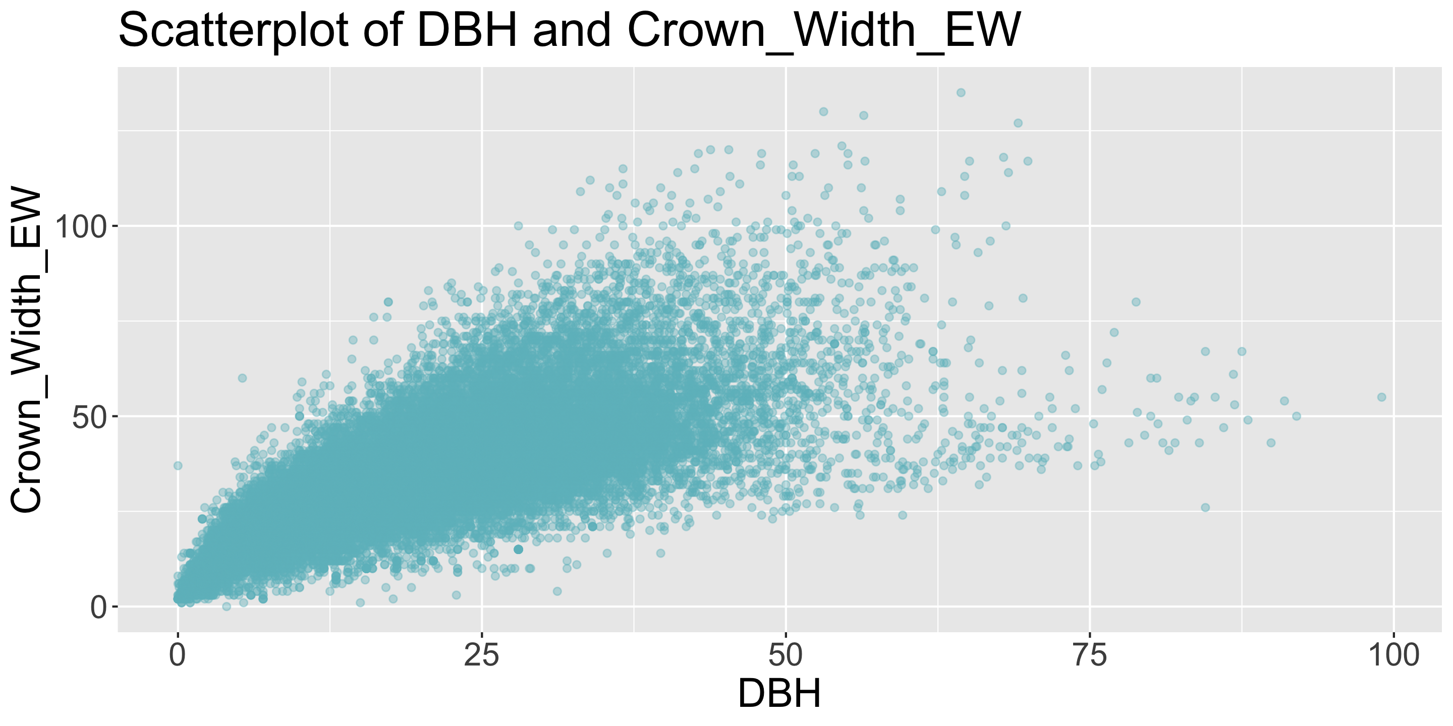
# Crown_Width_NS <dbl>, Crown_Width_EW <dbl>, Crown_Base_Height <dbl>,
# Collected_By <chr>, Park <chr>, Scientific_Name <chr>,
# Functional_Type <chr>, Mature_Size <chr>, Native <chr>, Edible <chr>,
# Nuisance <chr>, Structural_Value <dbl>, Carbon_Storage_lb <dbl>,
# Carbon_Storage_value <dbl>, Carbon_Sequestration_lb <dbl>, …