Data Wrangling & Summarization

Kelly McConville

Stat 100
Week 3 | Fall 2023

Announcements

With COVID working its way through campus right now, make sure to check the Sections spreadsheet and the Office hours spreadsheet for updates!
Let’s go through up to upload the pngs of your postcards to the RStudio Server on Posit Cloud.

Goals for Today

Consider measures for summarizing quantitative data
- Center
- Spread/variability
Consider measures for summarizing categorical data

Define data wrangling
Learn to use functions in the dplyr package to summarize and wrangle data

Load Necessary Packages

dplyr is part of this collection of data science packages.

# Load necessary packages
library(tidyverse)

Import the Data

july_2019 <- read_csv("data/july_2019.csv")

# Inspect the data
glimpse(july_2019)

Rows: 192
Columns: 8
$ DateTime  <chr> "07/04/2019 12:00:00 AM", "07/04/2019 12:15:00 AM", "07/04/2…
$ Day       <chr> "Thursday", "Thursday", "Thursday", "Thursday", "Thursday", …
$ Date      <date> 2019-07-04, 2019-07-04, 2019-07-04, 2019-07-04, 2019-07-04,…
$ Time      <time> 00:00:00, 00:15:00, 00:30:00, 00:45:00, 01:00:00, 01:15:00,…
$ Total     <dbl> 2, 3, 2, 0, 3, 2, 1, 0, 0, 0, 0, 0, 1, 1, 0, 0, 0, 0, 1, 1, …
$ Westbound <dbl> 2, 3, 1, 0, 2, 2, 1, 0, 0, 0, 0, 0, 1, 1, 0, 0, 0, 0, 0, 1, …
$ Eastbound <dbl> 0, 0, 1, 0, 1, 0, 0, 0, 0, 0, 0, 0, 0, 0, 0, 0, 0, 0, 1, 0, …
$ Occasion  <chr> "Fourth of July", "Fourth of July", "Fourth of July", "Fourt…

Summarizing Data

DateTime	Day	Date	Time	Total	Westbound	Eastbound	Occasion
07/04/2019 06:00:00 AM	Thursday	2019-07-04	06:00:00	1	1	0	Fourth of July
07/04/2019 06:15:00 AM	Thursday	2019-07-04	06:15:00	4	0	4	Fourth of July
07/04/2019 06:30:00 AM	Thursday	2019-07-04	06:30:00	9	1	8	Fourth of July
07/04/2019 06:45:00 AM	Thursday	2019-07-04	06:45:00	5	0	5	Fourth of July
07/04/2019 07:00:00 AM	Thursday	2019-07-04	07:00:00	3	3	0	Fourth of July
07/04/2019 07:15:00 AM	Thursday	2019-07-04	07:15:00	2	0	2	Fourth of July
07/04/2019 07:30:00 AM	Thursday	2019-07-04	07:30:00	5	2	3	Fourth of July
07/04/2019 07:45:00 AM	Thursday	2019-07-04	07:45:00	2	0	2	Fourth of July

Hard to do by eyeballing a spreadsheet with many rows!

Summarizing Data Visually

For a quantitative variable, want to answer:

What is an average value?
What is the trend/shape of the variable?
How much variation is there from case to case?

Need to learn key summary statistics: Numerical values computed based on the observed cases.

Measures of Center

Mean: Average of all the observations

\(n\) = Number of cases (sample size)
\(x_i\) = value of the i-th observation
Denote by \(\bar{x}\)

\[ \bar{x} = \frac{1}{n} \sum_{i = 1}^n x_i \]

# Test out on first 6 values
head(july_2019$Total)

[1] 2 3 2 0 3 2

Compute with a dplyr function:

summarize(july_2019, mean_bikes = mean(Total))

# A tibble: 1 × 1
  mean_bikes
       <dbl>
1       17.1

Measures of Center

Median: Middle value

Half of the data falls below the median
Denote by \(m\)
If \(n\) is even, then it is the average of the middle two values

# Test out on first 6 values
head(july_2019$Total)

[1] 2 3 2 0 3 2

Compute with a dplyr function:

summarize(july_2019, median_bikes = median(Total))

# A tibble: 1 × 1
  median_bikes
         <dbl>
1           11

Measures of Center

Why is the mean larger than the median?

summarize(july_2019, mean_bikes = mean(Total),
          median_bikes = median(Total))

# A tibble: 1 × 2
  mean_bikes median_bikes
       <dbl>        <dbl>
1       17.1           11

Computing Measures of Center by Groups

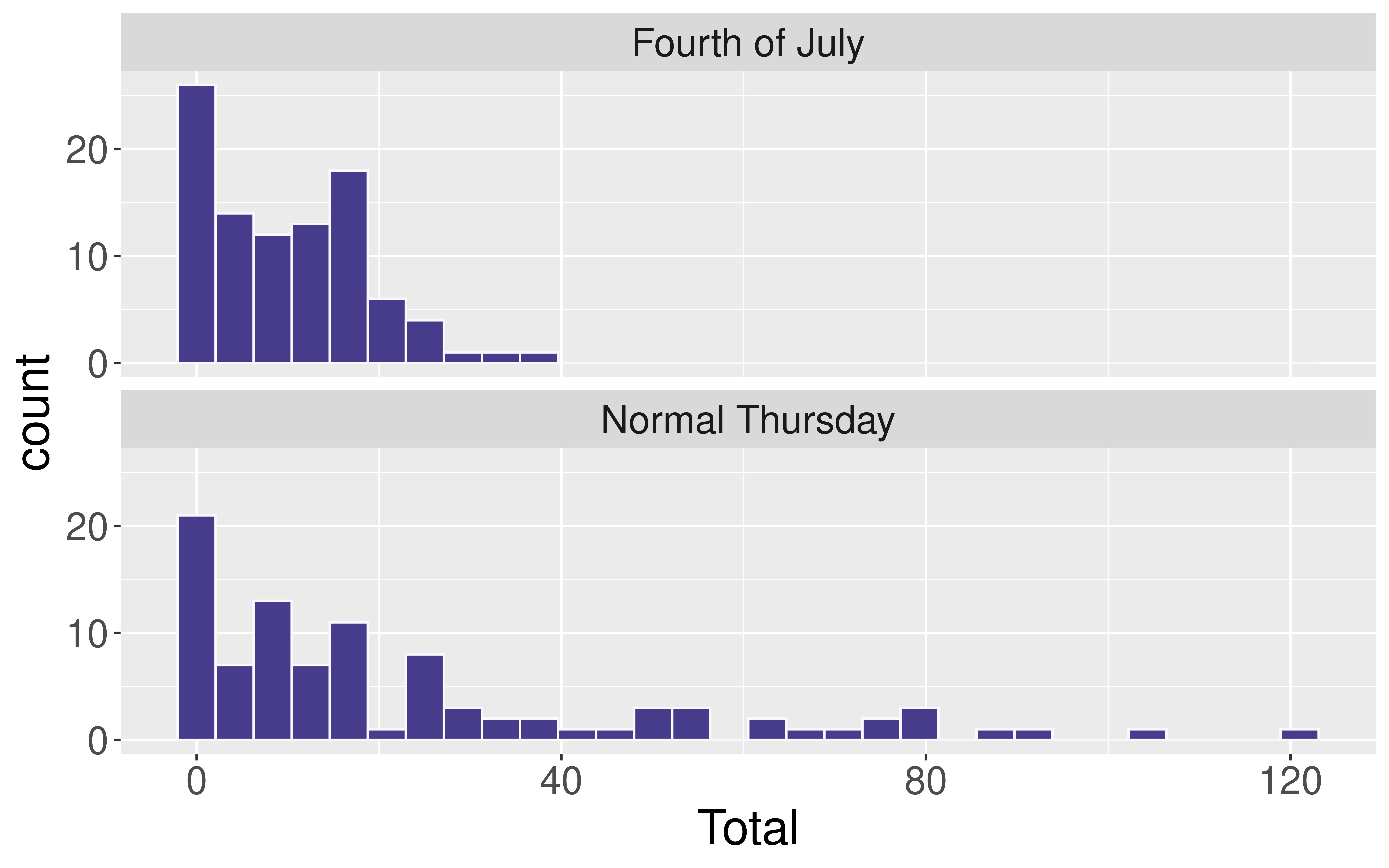
Question: Were there more bikes, on average, for Fourth of July or for the normal Thursday?

Computing Measures of Center by Groups

Handy dplyr function: group_by()

july_2019_grouped <- group_by(july_2019, Occasion)
july_2019_grouped

# A tibble: 192 × 8
# Groups:   Occasion [2]
   DateTime            Day   Date       Time  Total Westbound Eastbound Occasion
   <chr>               <chr> <date>     <tim> <dbl>     <dbl>     <dbl> <chr>   
 1 07/04/2019 12:00:0… Thur… 2019-07-04 00:00     2         2         0 Fourth …
 2 07/04/2019 12:15:0… Thur… 2019-07-04 00:15     3         3         0 Fourth …
 3 07/04/2019 12:30:0… Thur… 2019-07-04 00:30     2         1         1 Fourth …
 4 07/04/2019 12:45:0… Thur… 2019-07-04 00:45     0         0         0 Fourth …
 5 07/04/2019 01:00:0… Thur… 2019-07-04 01:00     3         2         1 Fourth …
 6 07/04/2019 01:15:0… Thur… 2019-07-04 01:15     2         2         0 Fourth …
 7 07/04/2019 01:30:0… Thur… 2019-07-04 01:30     1         1         0 Fourth …
 8 07/04/2019 01:45:0… Thur… 2019-07-04 01:45     0         0         0 Fourth …
 9 07/04/2019 02:00:0… Thur… 2019-07-04 02:00     0         0         0 Fourth …
10 07/04/2019 02:15:0… Thur… 2019-07-04 02:15     0         0         0 Fourth …
# ℹ 182 more rows

Computing Measures of Center by Groups

Compute summary statistics on the grouped data frame:

july_2019_grouped <- group_by(july_2019, Occasion)
summarize(july_2019_grouped,
          mean_bikes = mean(Total),
          median_bikes = median(Total))

# A tibble: 2 × 3
  Occasion        mean_bikes median_bikes
  <chr>                <dbl>        <dbl>
1 Fourth of July        10.0          9  
2 Normal Thursday       24.2         14.5

And now it is time to learn the pipe: `%>%`

Chaining `dplyr` Operations

Instead of:

july_2019_grouped <- group_by(july_2019, Occasion)
summarize(july_2019_grouped,
          mean_bikes = mean(Total),
          median_bikes = median(Total))

# A tibble: 2 × 3
  Occasion        mean_bikes median_bikes
  <chr>                <dbl>        <dbl>
1 Fourth of July        10.0          9  
2 Normal Thursday       24.2         14.5

Use the pipe:

july_2019 %>%
  group_by(Occasion) %>%
  summarize(mean_bikes = mean(Total),
          median_bikes = median(Total))

# A tibble: 2 × 3
  Occasion        mean_bikes median_bikes
  <chr>                <dbl>        <dbl>
1 Fourth of July        10.0          9  
2 Normal Thursday       24.2         14.5

Why pipe?

You can also use |>, which is newer and often referred to as the “base R pipe.”

Measures of Variability

Want a statistic that captures how much observations deviate from the mean

Find how much each observation deviates from the mean.
Compute the average of the deviations.

\[ \frac{1}{n} \sum_{i = 1}^n (x_i - \bar{x}) \]

# Test out on first 6 values
head(july_2019$Total)

[1] 2 3 2 0 3 2

Problem?

Measures of Variability

Want a statistic that captures how much observations deviate from the mean

Here is my NEW proposal:

Find how much each observation deviates from the mean.
Compute the average of the squared deviations.

# Test out on first 6 values
head(july_2019$Total)

[1] 2 3 2 0 3 2

Measures of Variability

Want a statistic that captures how much observations deviate from the mean

Here is my ACTUAL formula:

Find how much each observation deviates from the mean.
Compute the (nearly) average of the squared deviations.
Called sample variance \(s^2\).

\[ s^2 = \frac{1}{n - 1} \sum_{i = 1}^n (x_i - \bar{x})^2 \]

Compute with a dplyr function:

summarize(july_2019, var_bikes = var(Total))

# A tibble: 1 × 1
  var_bikes
      <dbl>
1      454.

Measures of Variability

Want a statistic that captures how much observations deviate from the mean

Find how much each observation deviates from the mean.
Compute the (nearly) average of the squared deviations.
Called sample variance \(s^2\).
The square root of the sample variance is called the sample standard deviation \(s\).

\[ s = \sqrt{\frac{1}{n - 1} \sum_{i = 1}^n (x_i - \bar{x})^2} \]

Compute with a dplyr function:

summarize(july_2019, var_bikes = var(Total),
          sd_bikes = sd(Total))

# A tibble: 1 × 2
  var_bikes sd_bikes
      <dbl>    <dbl>
1      454.     21.3

Measures of Variability

In addition to the sample standard deviation and the sample variance, there is the sample interquartile range (IQR):

\[ \mbox{IQR} = \mbox{Q}_3 - \mbox{Q}_1 \]

Compute with a dplyr function:

summarize(july_2019, iqr_bikes = IQR(Total))

# A tibble: 1 × 1
  iqr_bikes
      <dbl>
1        16

Comparing Measures of Variability

Which is more robust to outliers, the IQR or \(s\)?
Which is more commonly used, the IQR or \(s\)?

july_2019 %>%
  group_by(Occasion) %>%
summarize(sd_bikes = sd(Total),
          iqr_bikes = IQR(Total))

# A tibble: 2 × 3
  Occasion        sd_bikes iqr_bikes
  <chr>              <dbl>     <dbl>
1 Fourth of July      8.30      14  
2 Normal Thursday    27.2       27.2

Summarizing Categorical Variables

Return to the Cambridge Dogs

Focus on the dogs with the 5 most common names

dogs <- read_csv("https://data.cambridgema.gov/api/views/sckh-3xyx/rows.csv")

# Useful wrangling that we will come back to
dogs_top5 <- dogs %>% 
  mutate(Breed = case_when(
                       Dog_Breed == "Mixed Breed" ~ "Mixed",
                       Dog_Breed != "Mixed Breed" ~ "Single")) %>%
  filter(Dog_Name %in% c("Luna", "Charlie", "Lucy", "Cooper", "Rosie" ))

Frequency Table

count(dogs_top5, Dog_Name)

# A tibble: 5 × 2
  Dog_Name     n
  <chr>    <int>
1 Charlie     35
2 Cooper      23
3 Lucy        25
4 Luna        41
5 Rosie       22

ggplot(data = dogs_top5, 
    mapping = aes(x = Dog_Name)) +
  geom_bar()

Frequency Table

count(dogs_top5, Dog_Name)

# A tibble: 5 × 2
  Dog_Name     n
  <chr>    <int>
1 Charlie     35
2 Cooper      23
3 Lucy        25
4 Luna        41
5 Rosie       22

count(dogs_top5, Dog_Name, sort = TRUE)

# A tibble: 5 × 2
  Dog_Name     n
  <chr>    <int>
1 Luna        41
2 Charlie     35
3 Lucy        25
4 Cooper      23
5 Rosie       22

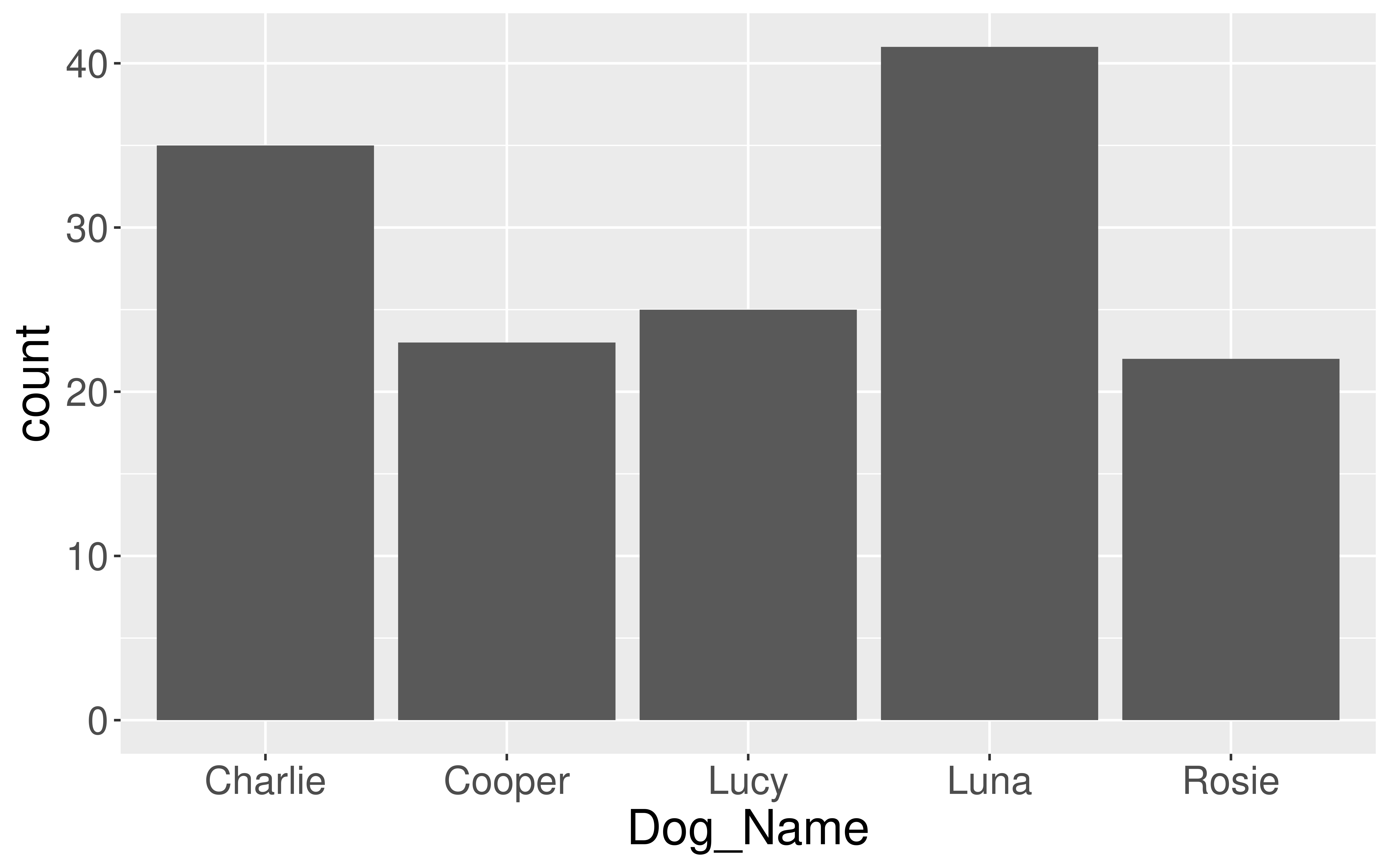
Another `ggplot2` `geom`: `geom_col()`

If you have already aggregated the data, you will use geom_col() instead of geom_bar().

dog_counts <- count(dogs_top5, Dog_Name)
dog_counts

# A tibble: 5 × 2
  Dog_Name     n
  <chr>    <int>
1 Charlie     35
2 Cooper      23
3 Lucy        25
4 Luna        41
5 Rosie       22

ggplot(data = dog_counts,
       mapping = aes(x = Dog_Name,
                     y = n)) +
  geom_col()

Another `ggplot2` `geom`: `geom_col()`

And use fct_reorder() instead of fct_infreq() to reorder bars.

dog_counts <- count(dogs_top5, Dog_Name)
dog_counts

# A tibble: 5 × 2
  Dog_Name     n
  <chr>    <int>
1 Charlie     35
2 Cooper      23
3 Lucy        25
4 Luna        41
5 Rosie       22

ggplot(data = dog_counts,
       mapping = aes(x = fct_reorder(Dog_Name, n),
                     y = n)) +
  geom_col()

Contingency Table

count(dogs_top5, Dog_Name, Breed)

# A tibble: 10 × 3
   Dog_Name Breed      n
   <chr>    <chr>  <int>
 1 Charlie  Mixed     12
 2 Charlie  Single    23
 3 Cooper   Mixed      9
 4 Cooper   Single    14
 5 Lucy     Mixed     10
 6 Lucy     Single    15
 7 Luna     Mixed     16
 8 Luna     Single    25
 9 Rosie    Mixed      6
10 Rosie    Single    16

ggplot(data = dogs_top5, 
    mapping = aes(x = Dog_Name, fill = Breed)) +
  geom_bar(position = "dodge")

Conditional Proportions

Beyond raw counts, we often summarize categorical data with conditional proportions.
- Especially when looking for relationships!

ggplot(data = dogs_top5, 
    mapping = aes(x = Dog_Name, fill = Breed)) +
  geom_bar(position = "fill")

Conditional Proportions

count(dogs_top5, Dog_Name, Breed)

# A tibble: 10 × 3
   Dog_Name Breed      n
   <chr>    <chr>  <int>
 1 Charlie  Mixed     12
 2 Charlie  Single    23
 3 Cooper   Mixed      9
 4 Cooper   Single    14
 5 Lucy     Mixed     10
 6 Lucy     Single    15
 7 Luna     Mixed     16
 8 Luna     Single    25
 9 Rosie    Mixed      6
10 Rosie    Single    16

count(dogs_top5, Dog_Name, Breed) %>%
  group_by(Dog_Name) %>%
  mutate(prop = n/sum(n))

# A tibble: 10 × 4
# Groups:   Dog_Name [5]
   Dog_Name Breed      n  prop
   <chr>    <chr>  <int> <dbl>
 1 Charlie  Mixed     12 0.343
 2 Charlie  Single    23 0.657
 3 Cooper   Mixed      9 0.391
 4 Cooper   Single    14 0.609
 5 Lucy     Mixed     10 0.4  
 6 Lucy     Single    15 0.6  
 7 Luna     Mixed     16 0.390
 8 Luna     Single    25 0.610
 9 Rosie    Mixed      6 0.273
10 Rosie    Single    16 0.727

The dplyr function mutate() adds new column(s) to your data frame.

Conditional Proportions

count(dogs_top5, Dog_Name, Breed) %>%
  group_by(Dog_Name) %>%
  mutate(prop = n/sum(n))

# A tibble: 10 × 4
# Groups:   Dog_Name [5]
   Dog_Name Breed      n  prop
   <chr>    <chr>  <int> <dbl>
 1 Charlie  Mixed     12 0.343
 2 Charlie  Single    23 0.657
 3 Cooper   Mixed      9 0.391
 4 Cooper   Single    14 0.609
 5 Lucy     Mixed     10 0.4  
 6 Lucy     Single    15 0.6  
 7 Luna     Mixed     16 0.390
 8 Luna     Single    25 0.610
 9 Rosie    Mixed      6 0.273
10 Rosie    Single    16 0.727

count(dogs_top5, Dog_Name, Breed) %>%
  group_by(Breed) %>%
  mutate(prop = n/sum(n))

# A tibble: 10 × 4
# Groups:   Breed [2]
   Dog_Name Breed      n  prop
   <chr>    <chr>  <int> <dbl>
 1 Charlie  Mixed     12 0.226
 2 Charlie  Single    23 0.247
 3 Cooper   Mixed      9 0.170
 4 Cooper   Single    14 0.151
 5 Lucy     Mixed     10 0.189
 6 Lucy     Single    15 0.161
 7 Luna     Mixed     16 0.302
 8 Luna     Single    25 0.269
 9 Rosie    Mixed      6 0.113
10 Rosie    Single    16 0.172

How does the interpretation change based on which variable you condition on?

Data Wrangling: Transformations done on the data

Why wrangle the data?

To summarize the data.

→ To compute the mean and standard deviation of the bike counts.

To drop missing values. (Need to be careful here!)

→ On our P-Set 2, we will see that ggplot2 will often drop observations before creating a graph.

To filter to a particular subset of the data.

→ To subset the bike counts data to 2 days in July of 2019.

To collapse the categories of a categorical variable.

→ To go from 86 dog breeds to just mixed or single breed.

Data Wrangling: Transformations done on the data

Why wrangle the data?

To arrange the data to make it easier to display.

→ To sort from most common dog name to least common.

To fix how R stores a variable.

→ For the bike data, I converted Day from a character variable/vector to a date variable/vector.

→ To join data frames when information about your cases is stored in multiple places!

Will see examples of this next class!

dplyr for Data Wrangling

Seven common wrangling verbs:
- summarize()
- count()
- mutate()
- select()
- filter()
- arrange()
- ---_join()
One action:
- group_by()

Return to `mutate()`

Add new variables

count(dogs_top5, Dog_Name, Breed) %>%
  group_by(Dog_Name) %>%
  mutate(prop = n/sum(n))

# A tibble: 10 × 4
# Groups:   Dog_Name [5]
   Dog_Name Breed      n  prop
   <chr>    <chr>  <int> <dbl>
 1 Charlie  Mixed     12 0.343
 2 Charlie  Single    23 0.657
 3 Cooper   Mixed      9 0.391
 4 Cooper   Single    14 0.609
 5 Lucy     Mixed     10 0.4  
 6 Lucy     Single    15 0.6  
 7 Luna     Mixed     16 0.390
 8 Luna     Single    25 0.610
 9 Rosie    Mixed      6 0.273
10 Rosie    Single    16 0.727

Modify existing variables

class(july_2019$DateTime)

[1] "character"

july_2019 <- july_2019 %>%
  mutate(DateTime = mdy_hms(DateTime))
class(july_2019$DateTime)

[1] "POSIXct" "POSIXt"

`select()`: Extract variables

dogs %>%
  select(Dog_Name, Dog_Breed)

# A tibble: 3,942 × 2
   Dog_Name       Dog_Breed                 
   <chr>          <chr>                     
 1 Butch          Mixed Breed               
 2 Baxter         Mixed Breed               
 3 Bodhi          Golden Retriever          
 4 Ocean          Pug                       
 5 Coco           Pug                       
 6 Brio           LABRADOODLE               
 7 Jolene Almeida German Shorthaired Pointer
 8 Ruger          Labrador Retriever        
 9 FLASH          Border Collie             
10 Leo            French Bulldog            
# ℹ 3,932 more rows

Motivation for `filter()`

count(dogs, Dog_Name, sort = TRUE)

# A tibble: 2,332 × 2
   Dog_Name     n
   <chr>    <int>
 1 Luna        41
 2 Charlie     35
 3 Lucy        25
 4 Cooper      23
 5 Rosie       22
 6 Olive       21
 7 Pepper      20
 8 Teddy       19
 9 Coco        18
10 Lola        17
# ℹ 2,322 more rows

`filter()`: Extract cases

dogs_top5 <- dogs %>% 
  filter(Dog_Name %in% c("Luna", "Charlie", "Lucy", "Cooper", "Rosie" ))

count(dogs_top5, Dog_Name, sort = TRUE)

# A tibble: 5 × 2
  Dog_Name     n
  <chr>    <int>
1 Luna        41
2 Charlie     35
3 Lucy        25
4 Cooper      23
5 Rosie       22

`arrange()`: Sort the cases

count(dogs_top5, Dog_Name) %>%
  arrange(n)

# A tibble: 5 × 2
  Dog_Name     n
  <chr>    <int>
1 Rosie       22
2 Cooper      23
3 Lucy        25
4 Charlie     35
5 Luna        41

count(dogs_top5, Dog_Name) %>%
  arrange(desc(n))

# A tibble: 5 × 2
  Dog_Name     n
  <chr>    <int>
1 Luna        41
2 Charlie     35
3 Lucy        25
4 Cooper      23
5 Rosie       22

count(dogs_top5, Dog_Name) %>%
  arrange(Dog_Name)

# A tibble: 5 × 2
  Dog_Name     n
  <chr>    <int>
1 Charlie     35
2 Cooper      23
3 Lucy        25
4 Luna        41
5 Rosie       22

Will see more data wrangling next week!

Reminders

With COVID working its way through campus right now, make sure to check the Sections spreadsheet and the Office hours spreadsheet for updates!

Announcements

Goals for Today

Load Necessary Packages

Import the Data

Summarizing Data

Summarizing Data Visually

Measures of Center

Measures of Center

Measures of Center

Computing Measures of Center by Groups

Computing Measures of Center by Groups

Computing Measures of Center by Groups

And now it is time to learn the pipe: %>%

Chaining dplyr Operations

Measures of Variability

Measures of Variability

Measures of Variability

Measures of Variability

Measures of Variability

Comparing Measures of Variability

Summarizing Categorical Variables

Return to the Cambridge Dogs

Frequency Table

Frequency Table

Another ggplot2 geom: geom_col()

Another ggplot2 geom: geom_col()

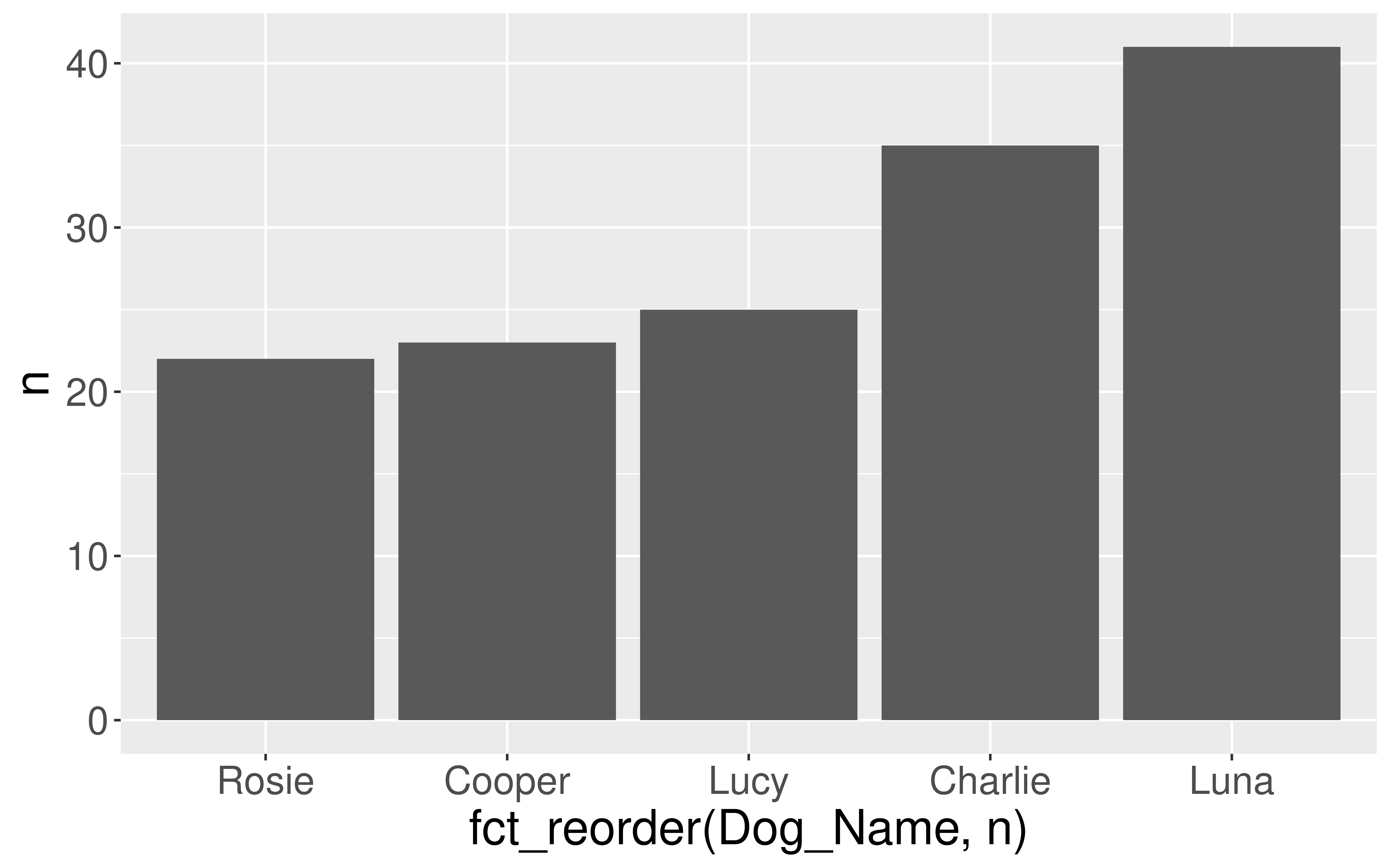
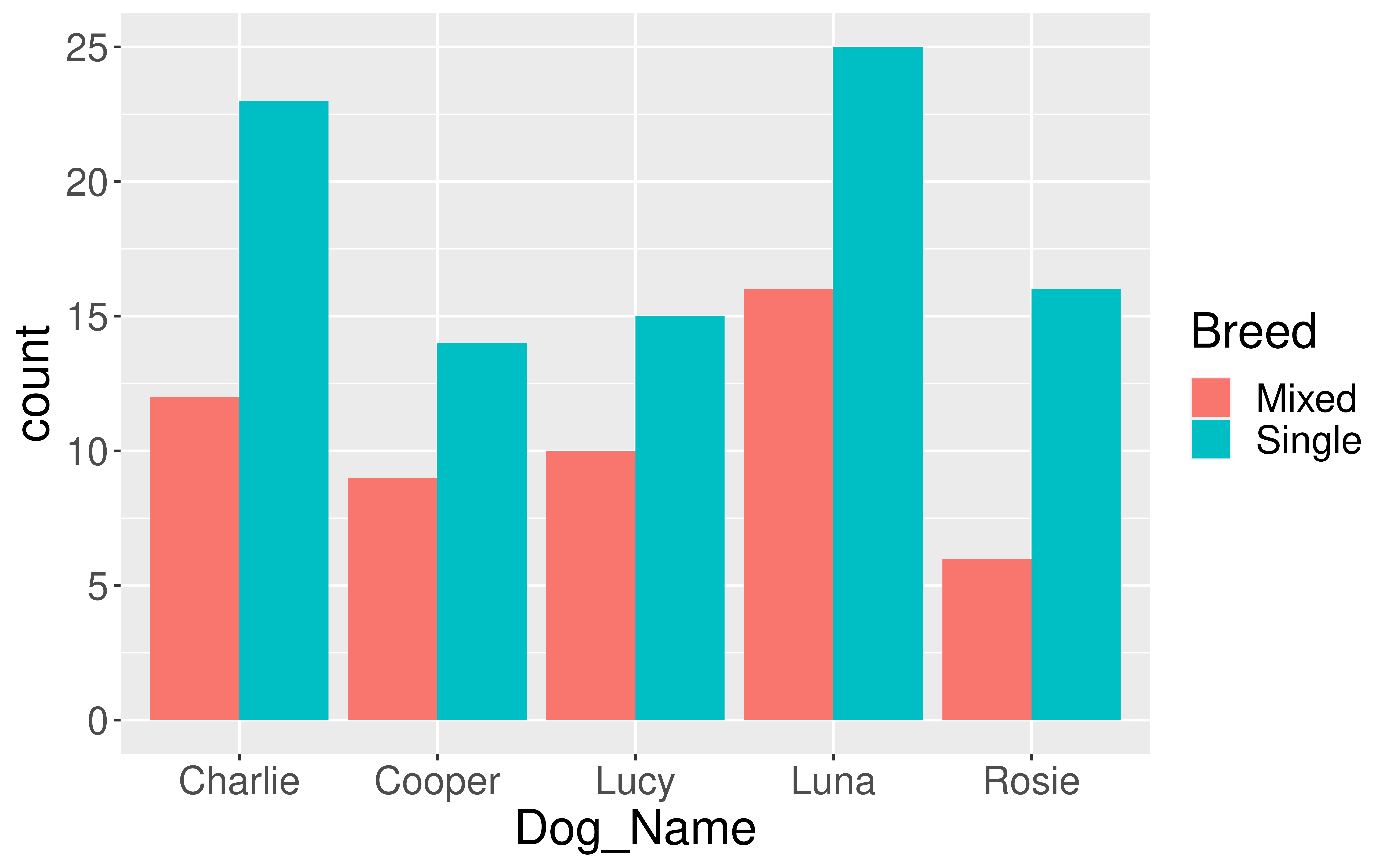
Contingency Table

Conditional Proportions

Conditional Proportions

Conditional Proportions

Data Wrangling: Transformations done on the data

Data Wrangling: Transformations done on the data

dplyr for Data Wrangling

Return to mutate()

select(): Extract variables

Motivation for filter()

filter(): Extract cases

arrange(): Sort the cases

Will see more data wrangling next week!

Reminders

And now it is time to learn the pipe: `%>%`

Chaining `dplyr` Operations

Another `ggplot2` `geom`: `geom_col()`

Another `ggplot2` `geom`: `geom_col()`

Return to `mutate()`

`select()`: Extract variables

Motivation for `filter()`

`filter()`: Extract cases

`arrange()`: Sort the cases