More Data Wrangling

Kelly McConville

Stat 100
Week 4 | Fall 2023

Announcements

Starting 1-on-1, virtual Office Hours
- 15 minute appointments, max 30 minutes per week
- For conceptual, not p-set, questions

Goals for Today

More data wrangling

Data joins

Load Necessary Packages

dplyr is part of this collection of data science packages.

# Load necessary packages
library(tidyverse)

Data Setting: Bureau of Labor Statistics (BLS) Consumer Expenditure Survey

BLS Mission: “Measures labor market activity, working conditions, price changes, and productivity in the U.S. economy to support public and private decision making.”

Data: Last quarter of the 2016 BLS Consumer Expenditure Survey.

library(tidyverse)

ce_raw <- read_csv("data/fmli.csv", 
                 na = c("NA", "."))
glimpse(ce_raw)

Rows: 6,301
Columns: 51
$ NEWID    <chr> "03324174", "03324204", "03324214", "03324244", "03324274", "…
$ PRINEARN <chr> "01", "01", "01", "01", "02", "01", "01", "01", "02", "01", "…
$ FINLWT21 <dbl> 25984.767, 6581.018, 20208.499, 18078.372, 20111.619, 19907.3…
$ FINCBTAX <dbl> 116920, 200, 117000, 0, 2000, 942, 0, 91000, 95000, 40037, 10…
$ BLS_URBN <dbl> 1, 1, 1, 1, 1, 1, 1, 1, 2, 1, 1, 1, 1, 1, 1, 1, 1, 1, 1, 1, 1…
$ POPSIZE  <dbl> 2, 3, 4, 2, 2, 2, 1, 2, 5, 2, 3, 2, 2, 3, 4, 3, 3, 1, 4, 1, 1…
$ EDUC_REF <chr> "16", "15", "16", "15", "14", "11", "10", "13", "12", "12", "…
$ EDUCA2   <dbl> 15, 15, 13, NA, NA, NA, NA, 15, 15, 14, 12, 12, NA, NA, NA, 1…
$ AGE_REF  <dbl> 63, 50, 47, 37, 51, 63, 77, 37, 51, 64, 26, 59, 81, 51, 67, 4…
$ AGE2     <dbl> 50, 47, 46, NA, NA, NA, NA, 36, 53, 67, 44, 62, NA, NA, NA, 4…
$ SEX_REF  <dbl> 1, 1, 2, 1, 2, 1, 2, 1, 1, 2, 2, 2, 2, 2, 2, 2, 2, 2, 1, 2, 1…
$ SEX2     <dbl> 2, 2, 1, NA, NA, NA, NA, 2, 2, 1, 1, 1, NA, NA, NA, 1, NA, 1,…
$ REF_RACE <dbl> 1, 4, 2, 1, 1, 1, 1, 1, 1, 1, 1, 1, 1, 1, 1, 2, 1, 1, 1, 1, 1…
$ RACE2    <dbl> 1, 4, 1, NA, NA, NA, NA, 1, 1, 1, 1, 1, NA, NA, NA, 2, NA, 1,…
$ HISP_REF <dbl> 2, 2, 2, 2, 2, 1, 1, 2, 2, 2, 2, 2, 2, 2, 2, 2, 2, 2, 2, 1, 1…
$ HISP2    <dbl> 2, 2, 1, NA, NA, NA, NA, 2, 2, 2, 2, 2, NA, NA, NA, 2, NA, 2,…
$ FAM_TYPE <dbl> 3, 4, 1, 8, 9, 9, 8, 3, 1, 1, 3, 1, 8, 9, 8, 5, 9, 4, 8, 3, 2…
$ MARITAL1 <dbl> 1, 1, 1, 5, 3, 3, 2, 1, 1, 1, 1, 1, 2, 3, 5, 1, 3, 1, 3, 1, 1…
$ REGION   <dbl> 4, 4, 3, 4, 4, 3, 4, 1, 3, 2, 1, 4, 1, 3, 3, 3, 2, 1, 2, 4, 3…
$ SMSASTAT <dbl> 1, 1, 1, 1, 1, 1, 1, 1, 2, 1, 1, 1, 1, 1, 1, 1, 1, 1, 1, 1, 1…
$ HIGH_EDU <chr> "16", "15", "16", "15", "14", "11", "10", "15", "15", "14", "…
$ EHOUSNGC <dbl> 0, 0, 0, 0, 0, 0, 0, 0, 0, 0, 0, 0, 0, 0, 0, 0, 0, 0, 0, 0, 0…
$ TOTEXPCQ <dbl> 0, 0, 0, 0, 0, 0, 0, 0, 0, 0, 0, 0, 0, 0, 0, 0, 0, 0, 0, 0, 0…
$ FOODCQ   <dbl> 0, 0, 0, 0, 0, 0, 0, 0, 0, 0, 0, 0, 0, 0, 0, 0, 0, 0, 0, 0, 0…
$ TRANSCQ  <dbl> 0, 0, 0, 0, 0, 0, 0, 0, 0, 0, 0, 0, 0, 0, 0, 0, 0, 0, 0, 0, 0…
$ HEALTHCQ <dbl> 0, 0, 0, 0, 0, 0, 0, 0, 0, 0, 0, 0, 0, 0, 0, 0, 0, 0, 0, 0, 0…
$ ENTERTCQ <dbl> 0, 0, 0, 0, 0, 0, 0, 0, 0, 0, 0, 0, 0, 0, 0, 0, 0, 0, 0, 0, 0…
$ EDUCACQ  <dbl> 0, 0, 0, 0, 0, 0, 0, 0, 0, 0, 0, 0, 0, 0, 0, 0, 0, 0, 0, 0, 0…
$ TOBACCCQ <dbl> 0, 0, 0, 0, 0, 0, 0, 0, 0, 0, 0, 0, 0, 0, 0, 0, 0, 0, 0, 0, 0…
$ STUDFINX <dbl> NA, NA, NA, NA, NA, NA, NA, NA, NA, NA, NA, NA, NA, NA, NA, N…
$ IRAX     <dbl> 1000000, 10000, 0, NA, NA, 0, 0, 15000, NA, 477000, NA, NA, N…
$ CUTENURE <dbl> 1, 1, 1, 1, 1, 2, 4, 1, 1, 2, 1, 2, 2, 2, 2, 4, 1, 1, 1, 4, 4…
$ FAM_SIZE <dbl> 4, 6, 2, 1, 2, 2, 1, 5, 2, 2, 4, 2, 1, 2, 1, 4, 2, 4, 1, 3, 3…
$ VEHQ     <dbl> 3, 5, 0, 4, 2, 0, 0, 2, 4, 2, 3, 2, 1, 3, 1, 2, 4, 4, 0, 2, 3…
$ ROOMSQ   <dbl> 8, 5, 6, 4, 4, 4, 7, 5, 4, 9, 6, 10, 4, 7, 5, 6, 6, 8, 18, 4,…
$ INC_HRS1 <dbl> 40, 40, 40, 44, 40, NA, NA, 40, 40, NA, 40, NA, NA, NA, NA, 4…
$ INC_HRS2 <dbl> 30, 40, 52, NA, NA, NA, NA, 40, 40, NA, 65, NA, NA, NA, NA, 6…
$ EARNCOMP <dbl> 3, 2, 2, 1, 4, 7, 8, 2, 2, 8, 2, 8, 8, 7, 8, 2, 7, 3, 1, 2, 1…
$ NO_EARNR <dbl> 4, 2, 2, 1, 2, 1, 0, 2, 2, 0, 2, 0, 0, 1, 0, 2, 1, 3, 1, 2, 1…
$ OCCUCOD1 <chr> "03", "03", "05", "03", "04", "", "", "12", "04", "", "01", "…
$ OCCUCOD2 <chr> "04", "02", "01", "", "", "", "", "02", "03", "", "11", "", "…
$ STATE    <chr> "41", "15", "48", "06", "06", "48", "06", "42", "", "27", "25…
$ DIVISION <dbl> 9, 9, 7, 9, 9, 7, 9, 2, NA, 4, 1, 8, 2, 5, 6, 7, 3, 2, 3, 9, …
$ TOTXEST  <dbl> 15452, 11459, 15738, 25978, 588, 0, 0, 7261, 9406, -1414, 141…
$ CREDFINX <dbl> 0, NA, 0, NA, 5, NA, NA, NA, NA, 0, NA, 0, NA, NA, NA, 2, 35,…
$ CREDITB  <dbl> NA, NA, NA, NA, NA, NA, NA, NA, NA, NA, NA, NA, NA, NA, NA, N…
$ CREDITX  <dbl> 4000, 5000, 2000, NA, 7000, 1800, NA, 6000, NA, 719, NA, 1200…
$ BUILDING <chr> "01", "01", "01", "02", "08", "01", "01", "01", "01", "01", "…
$ ST_HOUS  <dbl> 2, 2, 2, 2, 2, 2, 2, 2, 2, 2, 2, 2, 2, 2, 2, 2, 2, 2, 2, 2, 2…
$ INT_PHON <lgl> NA, NA, NA, NA, NA, NA, NA, NA, NA, NA, NA, NA, NA, NA, NA, N…
$ INT_HOME <lgl> NA, NA, NA, NA, NA, NA, NA, NA, NA, NA, NA, NA, NA, NA, NA, N…

Wrangling CE Data

Want to better understand a family’s income and expenditures

ce <- ce_raw %>%
  select(NEWID, PRINEARN, FINCBTAX,
         BLS_URBN, HIGH_EDU, TOTEXPCQ, IRAX)
dim(ce)

[1] 6301    7

Variables:

NEWID: ID for the household
PRINEARN: ID for which member of the household is the principal earner
FINCBTAX: Final income before taxes for the year

BLS_URBN: 1 = urban, 2 = rural
HIGH_EDU: Highest education in the household. 00 = Never attended, 10 = Grades 1-8, 11 = Grades 9-12, no degree, 12 = High school graduate, 13 = Some college, no degree, 14 = Associates degree, 15 = Bachelor’s degree, 16 = Masters, Professional/doctorate degree
TOTEXPCQ = Total household expenditures for the current quarter
IRAX = Total in retirement funds

Wrangling CE Data

ce <- ce %>%
  mutate(YEARLY_EXP = TOTEXPCQ*4)
ce

# A tibble: 6,301 × 8
   NEWID    PRINEARN FINCBTAX BLS_URBN HIGH_EDU TOTEXPCQ    IRAX YEARLY_EXP
   <chr>    <chr>       <dbl>    <dbl> <chr>       <dbl>   <dbl>      <dbl>
 1 03324174 01         116920        1 16              0 1000000          0
 2 03324204 01            200        1 15              0   10000          0
 3 03324214 01         117000        1 16              0       0          0
 4 03324244 01              0        1 15              0      NA          0
 5 03324274 02           2000        1 14              0      NA          0
 6 03324284 01            942        1 11              0       0          0
 7 03324294 01              0        1 10              0       0          0
 8 03324304 01          91000        1 15              0   15000          0
 9 03324324 02          95000        2 15              0      NA          0
10 03324334 01          40037        1 14              0  477000          0
# ℹ 6,291 more rows

Logical Operators

ce_sub <- ce %>%
  filter(YEARLY_EXP > 0, BLS_URBN == 1, HIGH_EDU != "00")
ce_sub

# A tibble: 3,950 × 8
   NEWID    PRINEARN FINCBTAX BLS_URBN HIGH_EDU TOTEXPCQ   IRAX YEARLY_EXP
   <chr>    <chr>       <dbl>    <dbl> <chr>       <dbl>  <dbl>      <dbl>
 1 03335204 01          37000        1 14          2492.      0      9968.
 2 03335214 01         103000        1 16          6128.     NA     24513.
 3 03335224 01          14686        1 13          1072.     NA      4287.
 4 03335244 02          33396        1 12          1630       0      6520 
 5 03335264 01              0        1 13          3213.     NA     12853.
 6 03335274 01              0        1 15          4674.      0     18694.
 7 03335294 01         745136        1 16          8693. 280000     34773.
 8 03335304 01          36000        1 16          3733.     NA     14933.
 9 03335314 02          45000        1 15          3627.   3000     14509 
10 03335334 01          20862        1 13           802.      0      3209.
# ℹ 3,940 more rows

Logical Operators

ce_sub <- ce %>%
  filter(YEARLY_EXP > 0, (BLS_URBN == 1 | HIGH_EDU != "00"))
ce_sub

# A tibble: 4,178 × 8
   NEWID    PRINEARN FINCBTAX BLS_URBN HIGH_EDU TOTEXPCQ   IRAX YEARLY_EXP
   <chr>    <chr>       <dbl>    <dbl> <chr>       <dbl>  <dbl>      <dbl>
 1 03335204 01          37000        1 14          2492.      0      9968.
 2 03335214 01         103000        1 16          6128.     NA     24513.
 3 03335224 01          14686        1 13          1072.     NA      4287.
 4 03335244 02          33396        1 12          1630       0      6520 
 5 03335264 01              0        1 13          3213.     NA     12853.
 6 03335274 01              0        1 15          4674.      0     18694.
 7 03335294 01         745136        1 16          8693. 280000     34773.
 8 03335304 01          36000        1 16          3733.     NA     14933.
 9 03335314 02          45000        1 15          3627.   3000     14509 
10 03335334 01          20862        1 13           802.      0      3209.
# ℹ 4,168 more rows

`case_when`: Recoding Variables

count(ce, BLS_URBN)

# A tibble: 2 × 2
  BLS_URBN     n
     <dbl> <int>
1        1  5952
2        2   349

ce <- ce %>%
  mutate(BLS_URBN = case_when(
    BLS_URBN == 1 ~ "Urban",
    BLS_URBN == 2 ~ "Rural"
  ))
count(ce, BLS_URBN)

# A tibble: 2 × 2
  BLS_URBN     n
  <chr>    <int>
1 Rural      349
2 Urban     5952

`case_when`: Creating Variables

count(ce, HIGH_EDU)

# A tibble: 8 × 2
  HIGH_EDU     n
  <chr>    <int>
1 00           8
2 10         110
3 11         302
4 12        1272
5 13        1297
6 14         714
7 15        1528
8 16        1070

ce <- ce %>%
  mutate(HIGH_EDU = as.numeric(HIGH_EDU))
count(ce, HIGH_EDU)

# A tibble: 8 × 2
  HIGH_EDU     n
     <dbl> <int>
1        0     8
2       10   110
3       11   302
4       12  1272
5       13  1297
6       14   714
7       15  1528
8       16  1070

ce <- ce %>%
  mutate(HIGH_EDU2 = case_when(
    is.na(HIGH_EDU) ~ NA,
    HIGH_EDU <= 11 ~ "Less than high school degree",
    between(HIGH_EDU, 12, 13) ~ "High school degree",
    HIGH_EDU >= 14 ~ "College degree"
  ))
count(ce, HIGH_EDU2)

# A tibble: 3 × 2
  HIGH_EDU2                        n
  <chr>                        <int>
1 College degree                3312
2 High school degree            2569
3 Less than high school degree   420

Variable Names

Sometimes datasets come with terrible variable names.

ce <- ce %>%
  rename(INCOME = FINCBTAX)
ce

# A tibble: 6,301 × 9
   NEWID PRINEARN INCOME BLS_URBN HIGH_EDU TOTEXPCQ    IRAX YEARLY_EXP HIGH_EDU2
   <chr> <chr>     <dbl> <chr>       <dbl>    <dbl>   <dbl>      <dbl> <chr>    
 1 0332… 01       116920 Urban          16        0 1000000          0 College …
 2 0332… 01          200 Urban          15        0   10000          0 College …
 3 0332… 01       117000 Urban          16        0       0          0 College …
 4 0332… 01            0 Urban          15        0      NA          0 College …
 5 0332… 02         2000 Urban          14        0      NA          0 College …
 6 0332… 01          942 Urban          11        0       0          0 Less tha…
 7 0332… 01            0 Urban          10        0       0          0 Less tha…
 8 0332… 01        91000 Urban          15        0   15000          0 College …
 9 0332… 02        95000 Rural          15        0      NA          0 College …
10 0332… 01        40037 Urban          14        0  477000          0 College …
# ℹ 6,291 more rows

Handling Missing Data

Want to compute mean income and mean retirement funds by location.

ce %>%
  group_by(BLS_URBN) %>%
  summarize(mean_INCOME = mean(INCOME),
            mean_IRAX = mean(IRAX),
            households = n())

# A tibble: 2 × 4
  BLS_URBN mean_INCOME mean_IRAX households
  <chr>          <dbl>     <dbl>      <int>
1 Rural         40440.        NA        349
2 Urban         63772.        NA       5952

ce_aggressive <- ce_raw %>%
  na.omit()
ce_aggressive

# A tibble: 0 × 51
# ℹ 51 variables: NEWID <chr>, PRINEARN <chr>, FINLWT21 <dbl>, FINCBTAX <dbl>,
#   BLS_URBN <dbl>, POPSIZE <dbl>, EDUC_REF <chr>, EDUCA2 <dbl>, AGE_REF <dbl>,
#   AGE2 <dbl>, SEX_REF <dbl>, SEX2 <dbl>, REF_RACE <dbl>, RACE2 <dbl>,
#   HISP_REF <dbl>, HISP2 <dbl>, FAM_TYPE <dbl>, MARITAL1 <dbl>, REGION <dbl>,
#   SMSASTAT <dbl>, HIGH_EDU <chr>, EHOUSNGC <dbl>, TOTEXPCQ <dbl>,
#   FOODCQ <dbl>, TRANSCQ <dbl>, HEALTHCQ <dbl>, ENTERTCQ <dbl>, EDUCACQ <dbl>,
#   TOBACCCQ <dbl>, STUDFINX <dbl>, IRAX <dbl>, CUTENURE <dbl>, …

Handling Missing Data

ce_moderate <- ce %>%
  drop_na(IRAX, INCOME, BLS_URBN) %>%
  group_by(BLS_URBN) %>%  
  summarize(mean_INCOME = mean(INCOME),
            mean_IRAX = mean(IRAX),
            households = n())

ce_moderate

# A tibble: 2 × 4
  BLS_URBN mean_INCOME mean_IRAX households
  <chr>          <dbl>     <dbl>      <int>
1 Rural         38651.    37008.         63
2 Urban         58987.    94512.        991

ce_light <- ce %>%
  group_by(BLS_URBN) %>%
  summarize(mean_INCOME = mean(INCOME, na.rm = TRUE),
            mean_IRAX = mean(IRAX, na.rm = TRUE), 
            households = n())

ce_light

# A tibble: 2 × 4
  BLS_URBN mean_INCOME mean_IRAX households
  <chr>          <dbl>     <dbl>      <int>
1 Rural         40440.    37008.        349
2 Urban         63772.    94512.       5952

Multiple Groupings

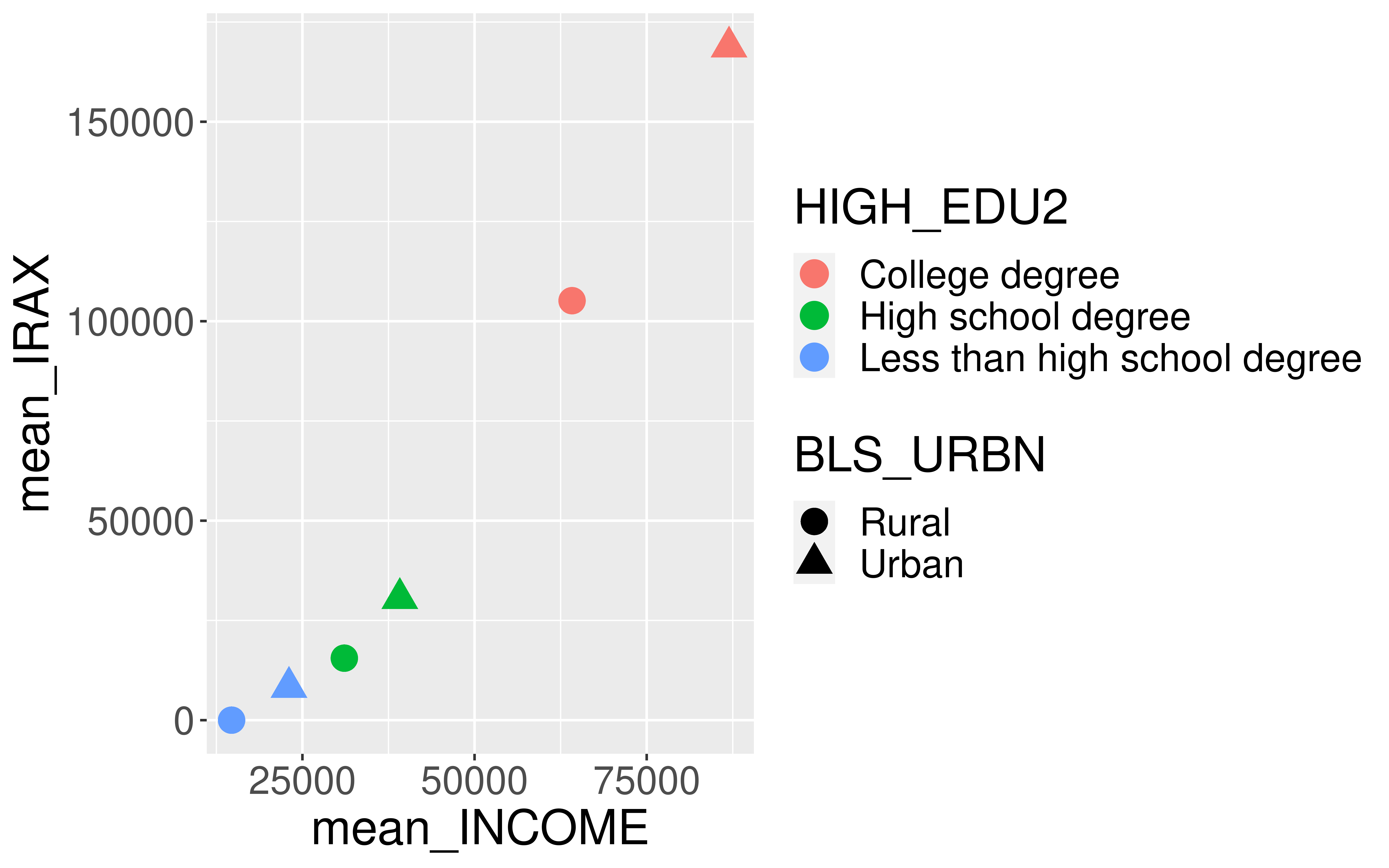
ce %>%
  group_by(BLS_URBN, HIGH_EDU2) %>%
  summarize(mean_INCOME = mean(INCOME, na.rm = TRUE),
            mean_IRAX = mean(IRAX, na.rm = TRUE), 
            households = n()) %>%
  arrange(mean_IRAX)

# A tibble: 6 × 5
# Groups:   BLS_URBN [2]
  BLS_URBN HIGH_EDU2                    mean_INCOME mean_IRAX households
  <chr>    <chr>                              <dbl>     <dbl>      <int>
1 Rural    Less than high school degree      14715.        0          39
2 Urban    Less than high school degree      23046.     8270.        381
3 Rural    High school degree                31087.    15543.        192
4 Urban    High school degree                39147.    30533.       2377
5 Rural    College degree                    64161.   105148.        118
6 Urban    College degree                    86957.   168767.       3194

Piping into `ggplot2`

ce %>%
  group_by(BLS_URBN, HIGH_EDU2) %>%
  summarize(mean_INCOME = mean(INCOME, na.rm = TRUE),
            mean_IRAX = mean(IRAX, na.rm = TRUE), 
            households = n()) %>%
  ggplot(mapping = aes(x = mean_INCOME,
                       y = mean_IRAX, 
                       shape = BLS_URBN,
                       color = HIGH_EDU2)) +
  geom_point(size = 5)

Data Joins

Often in the data analysis workflow, we have more than one data source, which means more than one dataframe, and we want to combine these dataframes.
Need principled way to combine.
- Need a key that links two dataframes together.
These multiple dataframes are called relational data.

CE Data

Household survey but data are also collected on individuals
- fmli: household data
- memi: household member-level data

fmli <- read_csv("data/fmli.csv", 
                 na = c("NA", ".")) %>%
  select(NEWID, PRINEARN, FINCBTAX,
         BLS_URBN, HIGH_EDU)
memi <- read_csv("data/memi.csv", 
                 na = c("NA", ".")) %>%
  select(NEWID, MEMBNO, AGE, SEX, EARNTYPE)

Want to add variables on the principal earner from the member data frame to the household data frame

CE Data

Key variable(s)?

fmli

# A tibble: 6,301 × 5
   NEWID    PRINEARN FINCBTAX BLS_URBN HIGH_EDU
   <chr>    <chr>       <dbl>    <dbl> <chr>   
 1 03324174 01         116920        1 16      
 2 03324204 01            200        1 15      
 3 03324214 01         117000        1 16      
 4 03324244 01              0        1 15      
 5 03324274 02           2000        1 14      
 6 03324284 01            942        1 11      
 7 03324294 01              0        1 10      
 8 03324304 01          91000        1 15      
 9 03324324 02          95000        2 15      
10 03324334 01          40037        1 14      
# ℹ 6,291 more rows

memi

# A tibble: 15,412 × 5
   NEWID    MEMBNO   AGE   SEX EARNTYPE
   <chr>     <dbl> <dbl> <dbl>    <dbl>
 1 03552611      1    58     2        2
 2 03552641      1    54     1        1
 3 03552641      2    49     2       NA
 4 03552651      1    39     2       NA
 5 03552651      2    10     2       NA
 6 03552651      3    32     1       NA
 7 03552651      4     7     1       NA
 8 03552651      5     9     1       NA
 9 03552681      1    38     1        3
10 03552681      2    34     2       NA
# ℹ 15,402 more rows

CE Data

Key variables?
- Problem with class?

class(fmli$NEWID)

[1] "character"

class(memi$NEWID)

[1] "character"

class(fmli$PRINEARN)

[1] "character"

class(memi$MEMBNO)

[1] "numeric"

CE Data

Key variables?
- Problem with class?

fmli <- mutate(fmli, PRINEARN = as.integer(PRINEARN))
class(fmli$PRINEARN)

[1] "integer"

class(memi$MEMBNO)

[1] "numeric"

CE Data

Want to add columns of memi to fmli that correspond to the principal earner’s memi data
- What type of join is that?

The World of Joins

Mutating joins: Add new variables to one dataset from matching observations in another.
- left_join() (and right_join())
- inner_join()
- full_join()
There are also filtering joins but we won’t cover those today.

Example Dataframes

Here I created the data frames by hand.

staff <- data.frame(member = c("Prof McConville", "Lety", "Kate",
                               "Thor", "Mally", "Dylan", "Nick"),
                 Year = c(2006, 2024, 2023, 2025, 2025, 2025, 2025),
                 Food = c("tikka masala", "chicken wings", "sushi",
                          "Sun HUDS Brunch", "quesadillas",
                          "shepards pie", "burgers"),
                 Neighborhood = c("Somerville", "River Central", "Quad", 
                                  "River East", "River Central",
                                  "Quad", "River Central"))
housing <- data.frame(Neighborhoods = c("Yard", "River East",
                                        "River Central", "River West",
                                        "Quad"),
                      Steps = c(75, 600, 450, 1100, 1200))

Example Dataframes

staff

           member Year            Food  Neighborhood
1 Prof McConville 2006    tikka masala    Somerville
2            Lety 2024   chicken wings River Central
3            Kate 2023           sushi          Quad
4            Thor 2025 Sun HUDS Brunch    River East
5           Mally 2025     quesadillas River Central
6           Dylan 2025    shepards pie          Quad
7            Nick 2025         burgers River Central

housing

  Neighborhoods Steps
1          Yard    75
2    River East   600
3 River Central   450
4    River West  1100
5          Quad  1200

`left_join()`

staff_new <- left_join(staff, housing)

Error in `left_join()`:
! `by` must be supplied when `x` and `y` have no common variables.
ℹ Use `cross_join()` to perform a cross-join.

staff_new

Error in eval(expr, envir, enclos): object 'staff_new' not found

`left_join()`

staff_new <- left_join(staff, housing, join_by("Neighborhood" == "Neighborhoods"))
staff_new

           member Year            Food  Neighborhood Steps
1 Prof McConville 2006    tikka masala    Somerville    NA
2            Lety 2024   chicken wings River Central   450
3            Kate 2023           sushi          Quad  1200
4            Thor 2025 Sun HUDS Brunch    River East   600
5           Mally 2025     quesadillas River Central   450
6           Dylan 2025    shepards pie          Quad  1200
7            Nick 2025         burgers River Central   450

`inner_join()`

staff_housing <- inner_join(staff, housing, join_by("Neighborhood" == "Neighborhoods"))
staff_housing

  member Year            Food  Neighborhood Steps
1   Lety 2024   chicken wings River Central   450
2   Kate 2023           sushi          Quad  1200
3   Thor 2025 Sun HUDS Brunch    River East   600
4  Mally 2025     quesadillas River Central   450
5  Dylan 2025    shepards pie          Quad  1200
6   Nick 2025         burgers River Central   450

`full_join()`

staff_housing <- full_join(staff, housing, join_by("Neighborhood" == "Neighborhoods"))
staff_housing

           member Year            Food  Neighborhood Steps
1 Prof McConville 2006    tikka masala    Somerville    NA
2            Lety 2024   chicken wings River Central   450
3            Kate 2023           sushi          Quad  1200
4            Thor 2025 Sun HUDS Brunch    River East   600
5           Mally 2025     quesadillas River Central   450
6           Dylan 2025    shepards pie          Quad  1200
7            Nick 2025         burgers River Central   450
8            <NA>   NA            <NA>          Yard    75
9            <NA>   NA            <NA>    River West  1100

Back to our Example

What kind of join do we want for the Consumer Expenditure data?
- Want to add columns of memi to fmli that correspond to the principal earner’s memi data
Also going to create smaller data frames for us to play with:

fmli_small <- filter(fmli, NEWID %in% c("03530051",
                                        "03327224",
                                        "03324324",
                                        "03324244"))
fmli_small

# A tibble: 4 × 5
  NEWID    PRINEARN FINCBTAX BLS_URBN HIGH_EDU
  <chr>       <int>    <dbl>    <dbl> <chr>   
1 03324244        1        0        1 15      
2 03324324        2    95000        2 15      
3 03327224        1        0        1 14      
4 03530051        3    70000        1 11

memi_small <- filter(memi, NEWID %in% c("03530051",
                                        "03327224",
                                        "03324324",
                                        "03324244"))
memi_small

# A tibble: 10 × 5
   NEWID    MEMBNO   AGE   SEX EARNTYPE
   <chr>     <dbl> <dbl> <dbl>    <dbl>
 1 03324244      1    37     1        1
 2 03324324      1    51     1        1
 3 03324324      2    53     2        1
 4 03327224      1    28     2        3
 5 03327224      2    32     1        2
 6 03327224      3     1     2       NA
 7 03530051      1    43     1       NA
 8 03530051      2    16     1       NA
 9 03530051      3    44     1        3
10 03530051      4     5     2       NA

Look at the Possible Joins

left_join(fmli_small, memi_small)

Joining with `by = join_by(NEWID)`

# A tibble: 10 × 9
   NEWID    PRINEARN FINCBTAX BLS_URBN HIGH_EDU MEMBNO   AGE   SEX EARNTYPE
   <chr>       <int>    <dbl>    <dbl> <chr>     <dbl> <dbl> <dbl>    <dbl>
 1 03324244        1        0        1 15            1    37     1        1
 2 03324324        2    95000        2 15            1    51     1        1
 3 03324324        2    95000        2 15            2    53     2        1
 4 03327224        1        0        1 14            1    28     2        3
 5 03327224        1        0        1 14            2    32     1        2
 6 03327224        1        0        1 14            3     1     2       NA
 7 03530051        3    70000        1 11            1    43     1       NA
 8 03530051        3    70000        1 11            2    16     1       NA
 9 03530051        3    70000        1 11            3    44     1        3
10 03530051        3    70000        1 11            4     5     2       NA

Look at the Possible Joins

Be careful. This erroneous example made my R crash when I tried it on the full data frames.

left_join(fmli_small, memi_small, join_by("PRINEARN" == "MEMBNO"))

# A tibble: 13 × 9
   NEWID.x  PRINEARN FINCBTAX BLS_URBN HIGH_EDU NEWID.y    AGE   SEX EARNTYPE
   <chr>       <dbl>    <dbl>    <dbl> <chr>    <chr>    <dbl> <dbl>    <dbl>
 1 03324244        1        0        1 15       03324244    37     1        1
 2 03324244        1        0        1 15       03324324    51     1        1
 3 03324244        1        0        1 15       03327224    28     2        3
 4 03324244        1        0        1 15       03530051    43     1       NA
 5 03324324        2    95000        2 15       03324324    53     2        1
 6 03324324        2    95000        2 15       03327224    32     1        2
 7 03324324        2    95000        2 15       03530051    16     1       NA
 8 03327224        1        0        1 14       03324244    37     1        1
 9 03327224        1        0        1 14       03324324    51     1        1
10 03327224        1        0        1 14       03327224    28     2        3
11 03327224        1        0        1 14       03530051    43     1       NA
12 03530051        3    70000        1 11       03327224     1     2       NA
13 03530051        3    70000        1 11       03530051    44     1        3

count(fmli_small, PRINEARN)

# A tibble: 3 × 2
  PRINEARN     n
     <int> <int>
1        1     2
2        2     1
3        3     1

count(memi_small, MEMBNO)

# A tibble: 4 × 2
  MEMBNO     n
   <dbl> <int>
1      1     4
2      2     3
3      3     2
4      4     1

Look at the Possible Joins

left_join(fmli_small, memi_small, join_by("NEWID" == "NEWID", "PRINEARN" == "MEMBNO"))

# A tibble: 4 × 8
  NEWID    PRINEARN FINCBTAX BLS_URBN HIGH_EDU   AGE   SEX EARNTYPE
  <chr>       <dbl>    <dbl>    <dbl> <chr>    <dbl> <dbl>    <dbl>
1 03324244        1        0        1 15          37     1        1
2 03324324        2    95000        2 15          53     2        1
3 03327224        1        0        1 14          28     2        3
4 03530051        3    70000        1 11          44     1        3

Look at the Possible Joins

inner_join(fmli_small, memi_small, join_by("NEWID" == "NEWID", "PRINEARN" == "MEMBNO"))

# A tibble: 4 × 8
  NEWID    PRINEARN FINCBTAX BLS_URBN HIGH_EDU   AGE   SEX EARNTYPE
  <chr>       <dbl>    <dbl>    <dbl> <chr>    <dbl> <dbl>    <dbl>
1 03324244        1        0        1 15          37     1        1
2 03324324        2    95000        2 15          53     2        1
3 03327224        1        0        1 14          28     2        3
4 03530051        3    70000        1 11          44     1        3

Why does this give us the same answer as left_join for this situation?

Look at the Possible Joins

full_join(fmli_small, memi_small, join_by("NEWID" == "NEWID", "PRINEARN" == "MEMBNO"))

# A tibble: 10 × 8
   NEWID    PRINEARN FINCBTAX BLS_URBN HIGH_EDU   AGE   SEX EARNTYPE
   <chr>       <dbl>    <dbl>    <dbl> <chr>    <dbl> <dbl>    <dbl>
 1 03324244        1        0        1 15          37     1        1
 2 03324324        2    95000        2 15          53     2        1
 3 03327224        1        0        1 14          28     2        3
 4 03530051        3    70000        1 11          44     1        3
 5 03324324        1       NA       NA <NA>        51     1        1
 6 03327224        2       NA       NA <NA>        32     1        2
 7 03327224        3       NA       NA <NA>         1     2       NA
 8 03530051        1       NA       NA <NA>        43     1       NA
 9 03530051        2       NA       NA <NA>        16     1       NA
10 03530051        4       NA       NA <NA>         5     2       NA

Joining Tips

fmli <- left_join(fmli, memi, join_by("NEWID" == "NEWID", "PRINEARN" == "MEMBNO"))

FIRST: conceptualize for yourself what you think you want the final dataset to look like!
Check initial dimensions and final dimensions.
Use variable names when joining even if they are the same.

Naming Wrangled Data

Should I name my new dataframe ce or ce1?

My answer:
- Is your new dataset structurally different? If so, give it a new name.
- Are you removing values you will need for a future analysis within the same document? If so, give it a new name.
- Are you just adding to or cleaning the data? If so, then write over the original.

Live Coding

Sage Advice from ModernDive

“Crucial: Unless you are very confident in what you are doing, it is worthwhile not starting to code right away. Rather, first sketch out on paper all the necessary data wrangling steps not using exact code, but rather high-level pseudocode that is informal yet detailed enough to articulate what you are doing. This way you won’t confuse what you are trying to do (the algorithm) with how you are going to do it (writing dplyr code).”

Announcements

Goals for Today

Load Necessary Packages

Data Setting: Bureau of Labor Statistics (BLS) Consumer Expenditure Survey

Wrangling CE Data

Wrangling CE Data

Logical Operators

Logical Operators

case_when: Recoding Variables

case_when: Creating Variables

Variable Names

Handling Missing Data

Handling Missing Data

Multiple Groupings

Piping into ggplot2

Data Joins

CE Data

CE Data

CE Data

CE Data

CE Data

The World of Joins

Example Dataframes

Example Dataframes

left_join()

left_join()

inner_join()

full_join()

Back to our Example

Look at the Possible Joins

Look at the Possible Joins

Look at the Possible Joins

Look at the Possible Joins

Look at the Possible Joins

Joining Tips

Naming Wrangled Data

Live Coding

Sage Advice from ModernDive

`case_when`: Recoding Variables

`case_when`: Creating Variables

Piping into `ggplot2`

`left_join()`

`left_join()`

`inner_join()`

`full_join()`