Data Collection

Kelly McConville

Stat 100
Week 4 | Fall 2023

Announcements

Oral practice in section this week.

Goals for Today

Finish up data joins.
Cover data collection/acquisition.

Getting Help with `R`

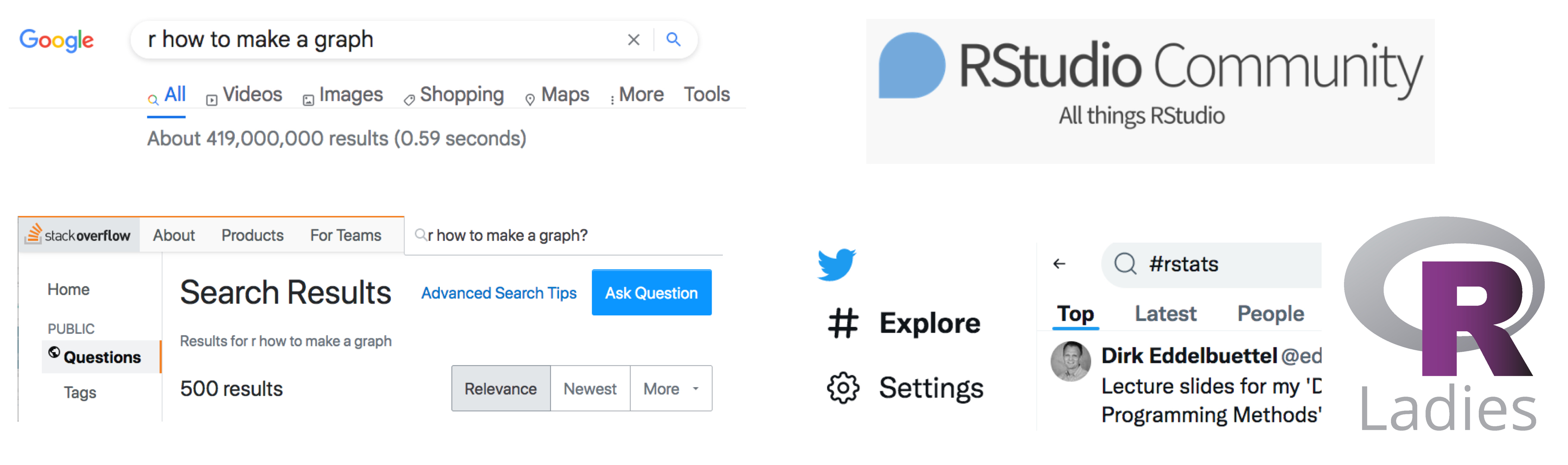
Novices asking the internet for R help = 😰
Get help from the Stat 100 teaching staff or classmates!
- Will start p-sets in section each week.
- Use the Slack #q-and-a channel.

Get help early before 😡 sets in!
- Be prepared for missing commas and quotes, capitalization issues, etc…
Later in the semester, will learn tricks for effectively getting R help online.

When to Get Help

😢 “I have no idea how to do this problem.”

→ Ask someone to point you to an similar example from the lecture, handouts, and guides.

→ Talk it through with someone on the Teaching Team or another Stat 100 student so together we can verbalize the process of going from Q to A.

😡 “I am getting a weird error but really think my code is correct/on the right track/matches the examples from class.”

→ It is time for a second pair of eyes. Don’t stare at the error for over 10 minutes.

🤩 And lots of other times too! 😬

When to Get Help

Remember:

→ Struggling is part of learning.

→ But let us help you ensure it is a productive struggle.

→ Struggling does NOT mean you are bad at stats!

Which Are YOU?

Data Visualizer

via GIPHY

Data Wrangler

via GIPHY

Load Necessary Packages

dplyr is part of this collection of data science packages.

# Load necessary packages
library(tidyverse)

Data Setting: Bureau of Labor Statistics (BLS) Consumer Expenditure Survey

BLS Mission: “Measures labor market activity, working conditions, price changes, and productivity in the U.S. economy to support public and private decision making.”

Data: Last quarter of the 2016 BLS Consumer Expenditure Survey.

library(tidyverse)

ce_raw <- read_csv("data/fmli.csv", 
                 na = c("NA", "."))
glimpse(ce_raw)

Rows: 6,301
Columns: 51
$ NEWID    <chr> "03324174", "03324204", "03324214", "03324244", "03324274", "…
$ PRINEARN <chr> "01", "01", "01", "01", "02", "01", "01", "01", "02", "01", "…
$ FINLWT21 <dbl> 25984.767, 6581.018, 20208.499, 18078.372, 20111.619, 19907.3…
$ FINCBTAX <dbl> 116920, 200, 117000, 0, 2000, 942, 0, 91000, 95000, 40037, 10…
$ BLS_URBN <dbl> 1, 1, 1, 1, 1, 1, 1, 1, 2, 1, 1, 1, 1, 1, 1, 1, 1, 1, 1, 1, 1…
$ POPSIZE  <dbl> 2, 3, 4, 2, 2, 2, 1, 2, 5, 2, 3, 2, 2, 3, 4, 3, 3, 1, 4, 1, 1…
$ EDUC_REF <chr> "16", "15", "16", "15", "14", "11", "10", "13", "12", "12", "…
$ EDUCA2   <dbl> 15, 15, 13, NA, NA, NA, NA, 15, 15, 14, 12, 12, NA, NA, NA, 1…
$ AGE_REF  <dbl> 63, 50, 47, 37, 51, 63, 77, 37, 51, 64, 26, 59, 81, 51, 67, 4…
$ AGE2     <dbl> 50, 47, 46, NA, NA, NA, NA, 36, 53, 67, 44, 62, NA, NA, NA, 4…
$ SEX_REF  <dbl> 1, 1, 2, 1, 2, 1, 2, 1, 1, 2, 2, 2, 2, 2, 2, 2, 2, 2, 1, 2, 1…
$ SEX2     <dbl> 2, 2, 1, NA, NA, NA, NA, 2, 2, 1, 1, 1, NA, NA, NA, 1, NA, 1,…
$ REF_RACE <dbl> 1, 4, 2, 1, 1, 1, 1, 1, 1, 1, 1, 1, 1, 1, 1, 2, 1, 1, 1, 1, 1…
$ RACE2    <dbl> 1, 4, 1, NA, NA, NA, NA, 1, 1, 1, 1, 1, NA, NA, NA, 2, NA, 1,…
$ HISP_REF <dbl> 2, 2, 2, 2, 2, 1, 1, 2, 2, 2, 2, 2, 2, 2, 2, 2, 2, 2, 2, 1, 1…
$ HISP2    <dbl> 2, 2, 1, NA, NA, NA, NA, 2, 2, 2, 2, 2, NA, NA, NA, 2, NA, 2,…
$ FAM_TYPE <dbl> 3, 4, 1, 8, 9, 9, 8, 3, 1, 1, 3, 1, 8, 9, 8, 5, 9, 4, 8, 3, 2…
$ MARITAL1 <dbl> 1, 1, 1, 5, 3, 3, 2, 1, 1, 1, 1, 1, 2, 3, 5, 1, 3, 1, 3, 1, 1…
$ REGION   <dbl> 4, 4, 3, 4, 4, 3, 4, 1, 3, 2, 1, 4, 1, 3, 3, 3, 2, 1, 2, 4, 3…
$ SMSASTAT <dbl> 1, 1, 1, 1, 1, 1, 1, 1, 2, 1, 1, 1, 1, 1, 1, 1, 1, 1, 1, 1, 1…
$ HIGH_EDU <chr> "16", "15", "16", "15", "14", "11", "10", "15", "15", "14", "…
$ EHOUSNGC <dbl> 0, 0, 0, 0, 0, 0, 0, 0, 0, 0, 0, 0, 0, 0, 0, 0, 0, 0, 0, 0, 0…
$ TOTEXPCQ <dbl> 0, 0, 0, 0, 0, 0, 0, 0, 0, 0, 0, 0, 0, 0, 0, 0, 0, 0, 0, 0, 0…
$ FOODCQ   <dbl> 0, 0, 0, 0, 0, 0, 0, 0, 0, 0, 0, 0, 0, 0, 0, 0, 0, 0, 0, 0, 0…
$ TRANSCQ  <dbl> 0, 0, 0, 0, 0, 0, 0, 0, 0, 0, 0, 0, 0, 0, 0, 0, 0, 0, 0, 0, 0…
$ HEALTHCQ <dbl> 0, 0, 0, 0, 0, 0, 0, 0, 0, 0, 0, 0, 0, 0, 0, 0, 0, 0, 0, 0, 0…
$ ENTERTCQ <dbl> 0, 0, 0, 0, 0, 0, 0, 0, 0, 0, 0, 0, 0, 0, 0, 0, 0, 0, 0, 0, 0…
$ EDUCACQ  <dbl> 0, 0, 0, 0, 0, 0, 0, 0, 0, 0, 0, 0, 0, 0, 0, 0, 0, 0, 0, 0, 0…
$ TOBACCCQ <dbl> 0, 0, 0, 0, 0, 0, 0, 0, 0, 0, 0, 0, 0, 0, 0, 0, 0, 0, 0, 0, 0…
$ STUDFINX <dbl> NA, NA, NA, NA, NA, NA, NA, NA, NA, NA, NA, NA, NA, NA, NA, N…
$ IRAX     <dbl> 1000000, 10000, 0, NA, NA, 0, 0, 15000, NA, 477000, NA, NA, N…
$ CUTENURE <dbl> 1, 1, 1, 1, 1, 2, 4, 1, 1, 2, 1, 2, 2, 2, 2, 4, 1, 1, 1, 4, 4…
$ FAM_SIZE <dbl> 4, 6, 2, 1, 2, 2, 1, 5, 2, 2, 4, 2, 1, 2, 1, 4, 2, 4, 1, 3, 3…
$ VEHQ     <dbl> 3, 5, 0, 4, 2, 0, 0, 2, 4, 2, 3, 2, 1, 3, 1, 2, 4, 4, 0, 2, 3…
$ ROOMSQ   <dbl> 8, 5, 6, 4, 4, 4, 7, 5, 4, 9, 6, 10, 4, 7, 5, 6, 6, 8, 18, 4,…
$ INC_HRS1 <dbl> 40, 40, 40, 44, 40, NA, NA, 40, 40, NA, 40, NA, NA, NA, NA, 4…
$ INC_HRS2 <dbl> 30, 40, 52, NA, NA, NA, NA, 40, 40, NA, 65, NA, NA, NA, NA, 6…
$ EARNCOMP <dbl> 3, 2, 2, 1, 4, 7, 8, 2, 2, 8, 2, 8, 8, 7, 8, 2, 7, 3, 1, 2, 1…
$ NO_EARNR <dbl> 4, 2, 2, 1, 2, 1, 0, 2, 2, 0, 2, 0, 0, 1, 0, 2, 1, 3, 1, 2, 1…
$ OCCUCOD1 <chr> "03", "03", "05", "03", "04", "", "", "12", "04", "", "01", "…
$ OCCUCOD2 <chr> "04", "02", "01", "", "", "", "", "02", "03", "", "11", "", "…
$ STATE    <chr> "41", "15", "48", "06", "06", "48", "06", "42", "", "27", "25…
$ DIVISION <dbl> 9, 9, 7, 9, 9, 7, 9, 2, NA, 4, 1, 8, 2, 5, 6, 7, 3, 2, 3, 9, …
$ TOTXEST  <dbl> 15452, 11459, 15738, 25978, 588, 0, 0, 7261, 9406, -1414, 141…
$ CREDFINX <dbl> 0, NA, 0, NA, 5, NA, NA, NA, NA, 0, NA, 0, NA, NA, NA, 2, 35,…
$ CREDITB  <dbl> NA, NA, NA, NA, NA, NA, NA, NA, NA, NA, NA, NA, NA, NA, NA, N…
$ CREDITX  <dbl> 4000, 5000, 2000, NA, 7000, 1800, NA, 6000, NA, 719, NA, 1200…
$ BUILDING <chr> "01", "01", "01", "02", "08", "01", "01", "01", "01", "01", "…
$ ST_HOUS  <dbl> 2, 2, 2, 2, 2, 2, 2, 2, 2, 2, 2, 2, 2, 2, 2, 2, 2, 2, 2, 2, 2…
$ INT_PHON <lgl> NA, NA, NA, NA, NA, NA, NA, NA, NA, NA, NA, NA, NA, NA, NA, N…
$ INT_HOME <lgl> NA, NA, NA, NA, NA, NA, NA, NA, NA, NA, NA, NA, NA, NA, NA, N…

CE Data

Household survey but data are also collected on individuals
- fmli: household data
- memi: household member-level data

fmli <- read_csv("data/fmli.csv", 
                 na = c("NA", ".")) %>%
  select(NEWID, PRINEARN, FINCBTAX,
         BLS_URBN, HIGH_EDU)
memi <- read_csv("data/memi.csv", 
                 na = c("NA", ".")) %>%
  select(NEWID, MEMBNO, AGE, SEX, EARNTYPE)

fmli <- mutate(fmli, PRINEARN = as.integer(PRINEARN))

Want to add variables on the principal earner from the member data frame to the household data frame

Smaller Sets of CE Data

fmli_small <- filter(fmli, NEWID %in% c("03530051",
                                        "03327224",
                                        "03324324",
                                        "03324244"))
fmli_small

# A tibble: 4 × 5
  NEWID    PRINEARN FINCBTAX BLS_URBN HIGH_EDU
  <chr>       <int>    <dbl>    <dbl> <chr>   
1 03324244        1        0        1 15      
2 03324324        2    95000        2 15      
3 03327224        1        0        1 14      
4 03530051        3    70000        1 11

memi_small <- filter(memi, NEWID %in% c("03530051",
                                        "03327224",
                                        "03324324",
                                        "03324244"))
memi_small

# A tibble: 10 × 5
   NEWID    MEMBNO   AGE   SEX EARNTYPE
   <chr>     <dbl> <dbl> <dbl>    <dbl>
 1 03324244      1    37     1        1
 2 03324324      1    51     1        1
 3 03324324      2    53     2        1
 4 03327224      1    28     2        3
 5 03327224      2    32     1        2
 6 03327224      3     1     2       NA
 7 03530051      1    43     1       NA
 8 03530051      2    16     1       NA
 9 03530051      3    44     1        3
10 03530051      4     5     2       NA

Look at the Possible Joins

full_join(fmli_small, memi_small, join_by("NEWID" == "NEWID", "PRINEARN" == "MEMBNO"))

# A tibble: 10 × 8
   NEWID    PRINEARN FINCBTAX BLS_URBN HIGH_EDU   AGE   SEX EARNTYPE
   <chr>       <dbl>    <dbl>    <dbl> <chr>    <dbl> <dbl>    <dbl>
 1 03324244        1        0        1 15          37     1        1
 2 03324324        2    95000        2 15          53     2        1
 3 03327224        1        0        1 14          28     2        3
 4 03530051        3    70000        1 11          44     1        3
 5 03324324        1       NA       NA <NA>        51     1        1
 6 03327224        2       NA       NA <NA>        32     1        2
 7 03327224        3       NA       NA <NA>         1     2       NA
 8 03530051        1       NA       NA <NA>        43     1       NA
 9 03530051        2       NA       NA <NA>        16     1       NA
10 03530051        4       NA       NA <NA>         5     2       NA

Joining Tips

fmli <- left_join(fmli, memi, join_by("NEWID" == "NEWID", "PRINEARN" == "MEMBNO"))

FIRST: conceptualize for yourself what you think you want the final dataset to look like!
Check initial dimensions and final dimensions.
Use variable names when joining even if they are the same.

Naming Wrangled Data

Should I name my new dataframe ce or ce1?

My answer:
- Is your new dataset structurally different? If so, give it a new name.
- Are you removing values you will need for a future analysis within the same document? If so, give it a new name.
- Are you just adding to or cleaning the data? If so, then write over the original.

Live Coding

Sage Advice from ModernDive

“Crucial: Unless you are very confident in what you are doing, it is worthwhile not starting to code right away. Rather, first sketch out on paper all the necessary data wrangling steps not using exact code, but rather high-level pseudocode that is informal yet detailed enough to articulate what you are doing. This way you won’t confuse what you are trying to do (the algorithm) with how you are going to do it (writing dplyr code).”

Now for Data Collection

Motivating Our Discussion of Data Collection

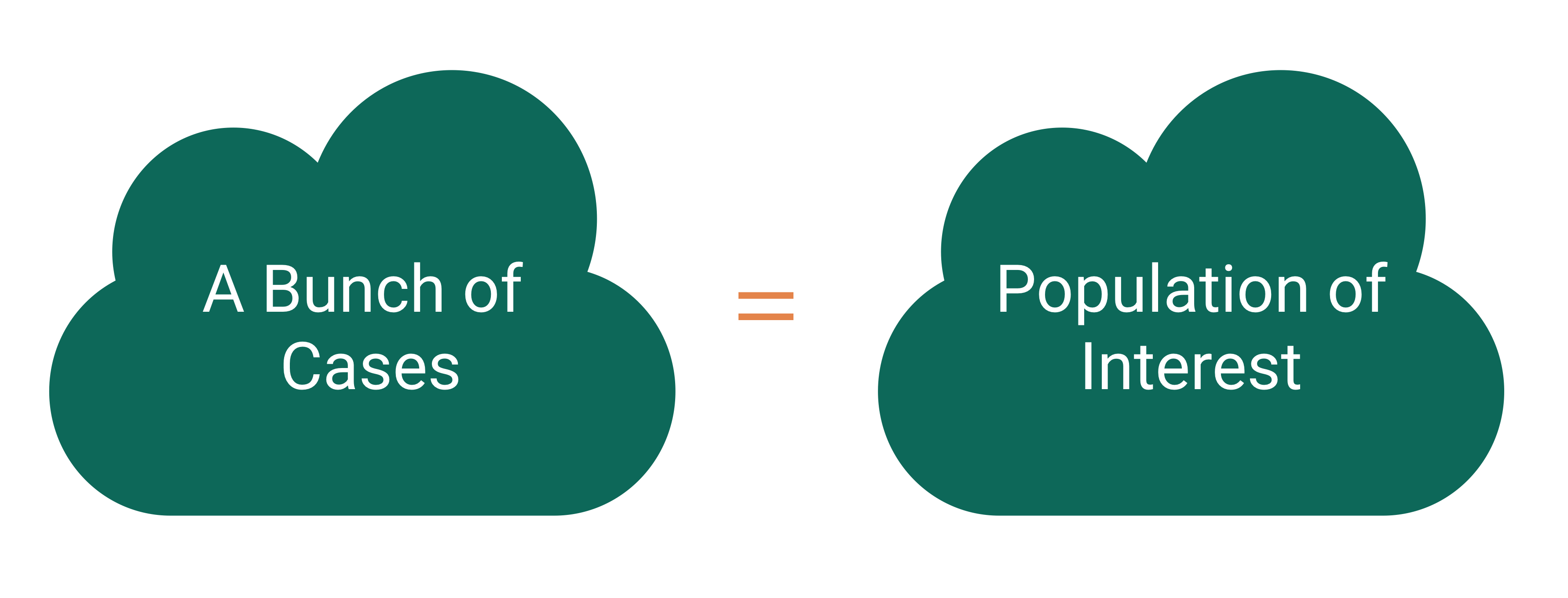
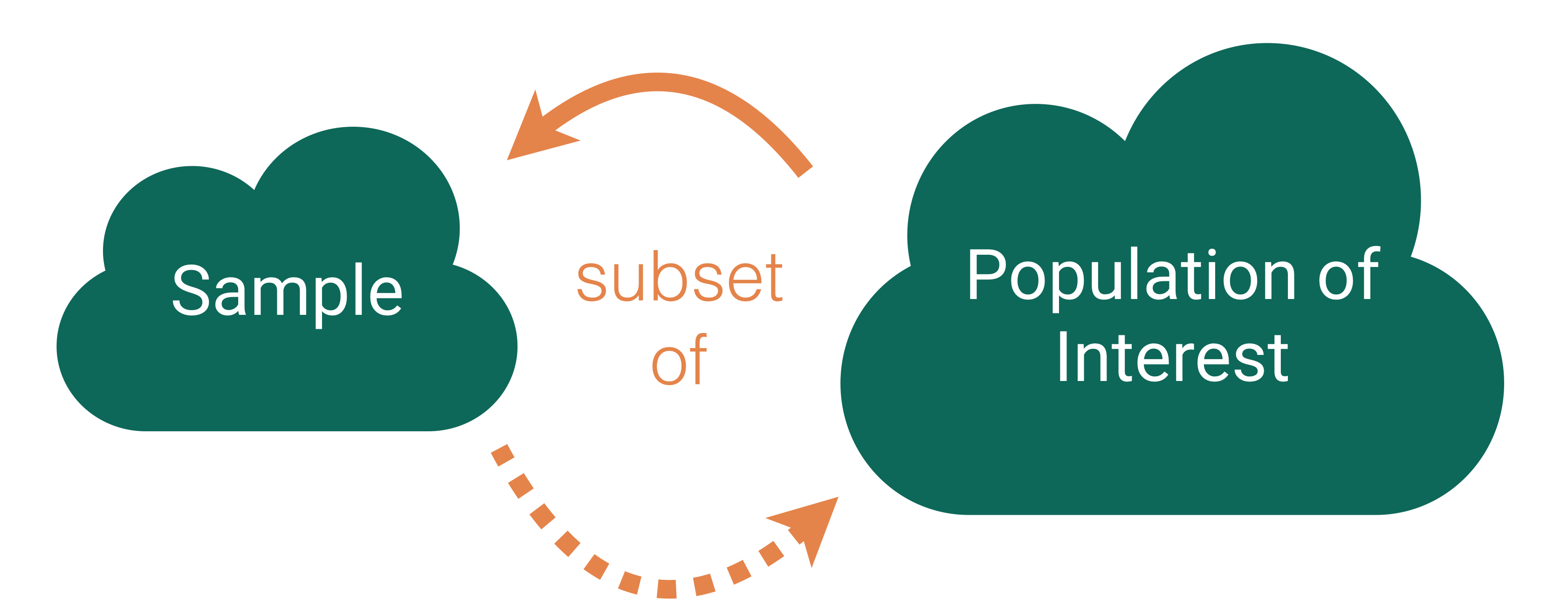
Who are the data supposed to represent?

Key questions:

What evidence is there that the data are representative?
Who is present? Who is absent?
Who is overrepresented? Who is underrepresented?

Who are the data supposed to represent?

Census: We have data on the whole population!

Who are the data supposed to represent?

Who are the data supposed to represent?

Key questions:

What evidence is there that the sample is representative of the population?
Who is present? Who is absent?
Who is overrepresented? Who is underrepresented?

Sampling Bias

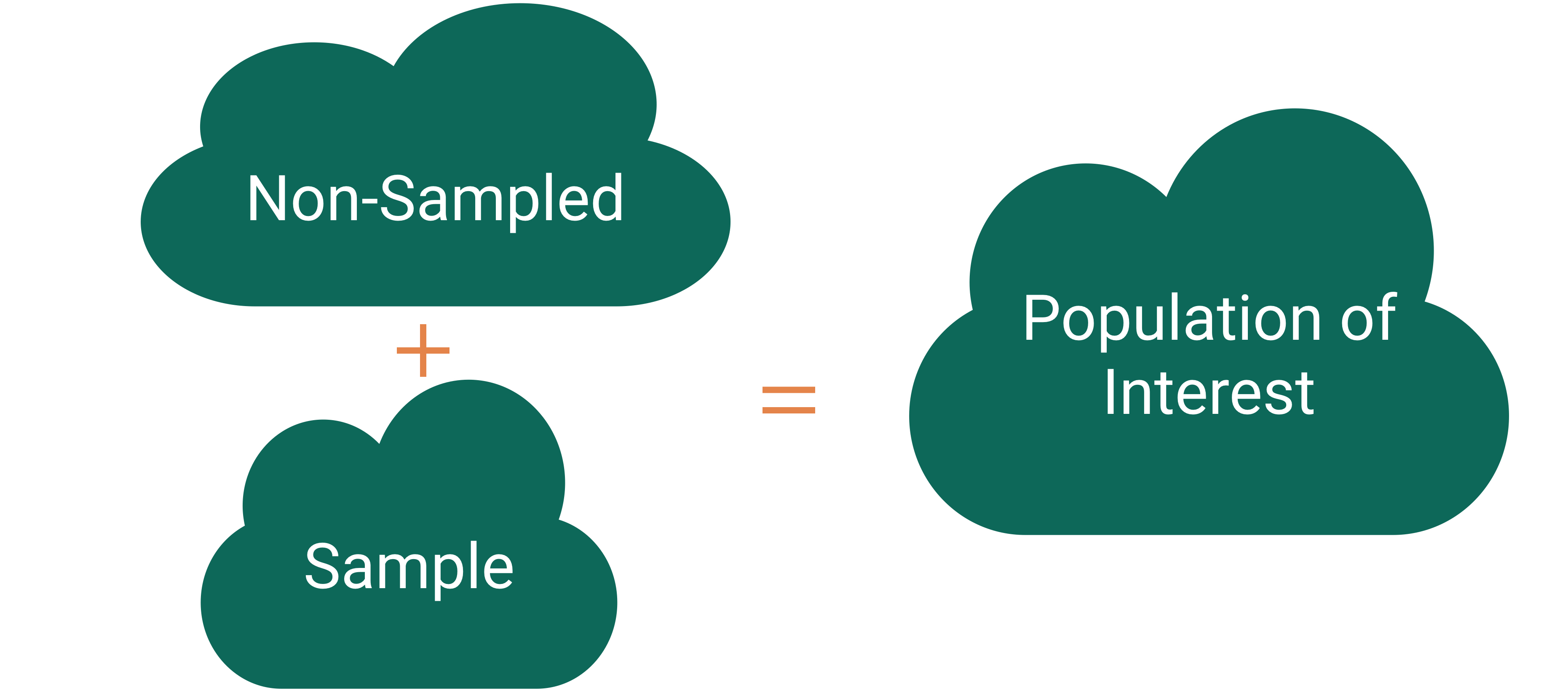
Sampling bias: When the sampled units are systematically different from the non-sampled units on the variables of interest.

Sampling Bias Example

The Literary Digest was a political magazine that correctly predicted the presidential outcomes from 1916 to 1932. In 1936, they conducted the most extensive (to that date) public opinion poll. They mailed questionnaires to over 10 million people (about 1/3 of US households) whose names and addresses they obtained from telephone books and vehicle registration lists.

Population of Interest:

Sample:

Sampling bias:

Random Sampling

Use random sampling (a random mechanism for selecting cases from the population) to remove sampling bias.

Types of random sampling

Simple random sampling
Cluster sampling
Stratified random sampling
Systematic sampling

Why aren’t all samples generated using simple random sampling?

US Forest Inventory and Analysis Program

Mission: “Make and keep current a comprehensive inventory and analysis of the present and prospective conditions of and requirements for the renewable resources of the forest and rangelands of the US.”

Need a random sample of ground plots to say something about the state of our nation’s forests!

FIA: Simple Random Sampling

Break the landscape up into equally sized plots (~1 acre).
Number each plot from 1 to 6,755,200.
Use a random mechanism to sample a plot for about every 6,000 acres.

sample(x = 1:6755200, size = 1126) %>%
  head()

[1] 5688519 3872920 5628952  427960 4873669 5295354

Thoughts on this sampling design?

FIA: Cluster Random Sampling

Break the landscape up into equally sized plots (~1 acre).
Put each plot in a cluster.
- For our example: cluster = county.
Number each cluster.
Use a random mechanism to sample 2 clusters.
Sample all plots in those 2 clusters.

sample(x = 1:14, size = 2)

[1] 1 3

Thoughts on this sampling design?

FIA: Cluster Random Sampling

Break the landscape up into equally sized plots (~1 acre).
Put each plot in a cluster.
- For our example: cluster = county.
Number each cluster.
Use a random mechanism to sample 2 clusters.
Take a simple random sample within the sampled clusters.

sample(x = 1:14, size = 2)

[1] 8 2

sample(x = 1:---, size = ---)

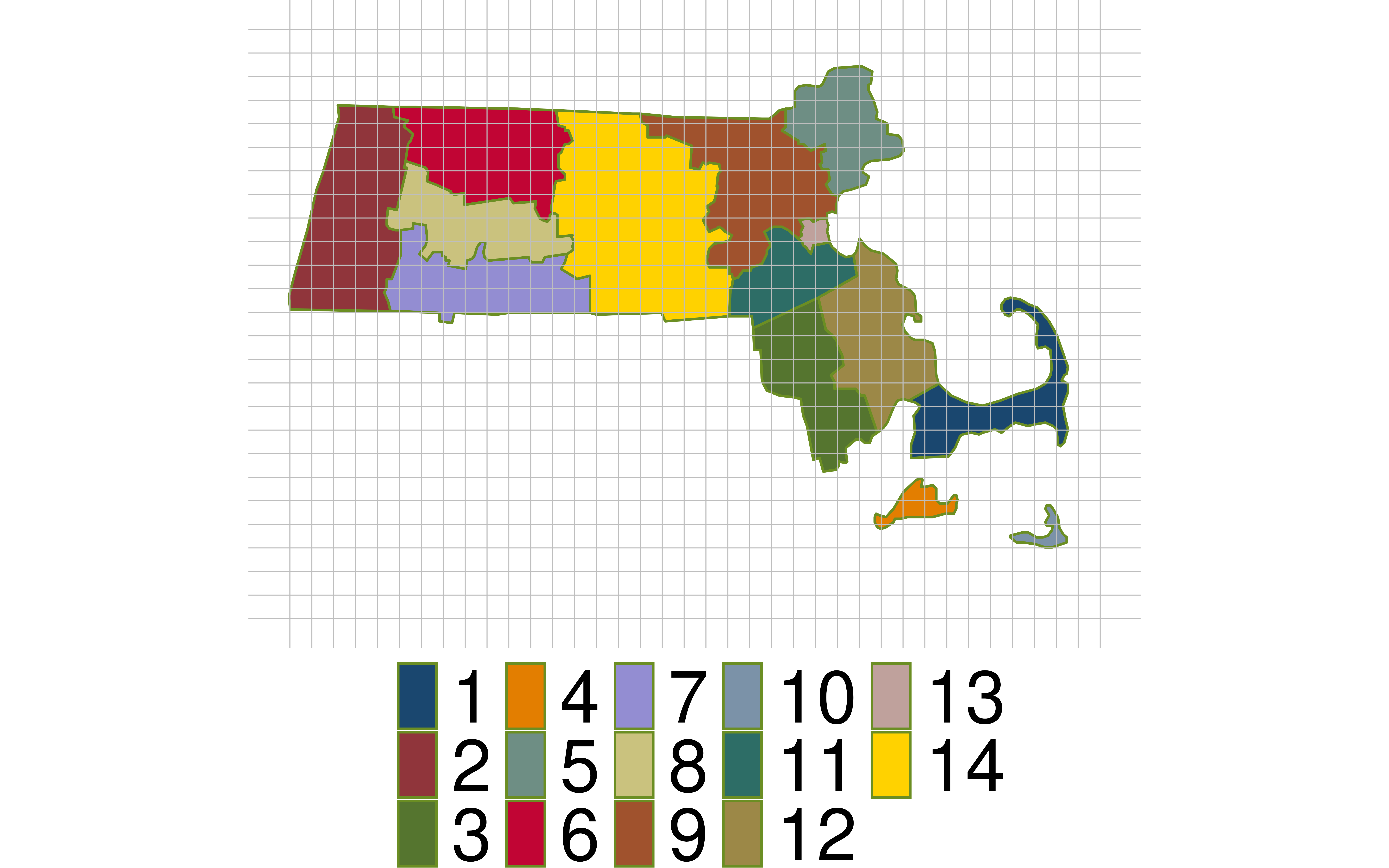
Subsampling within each sampled cluster is much more common than subsampling the whole sampled cluster!

FIA: Cluster Random Sampling

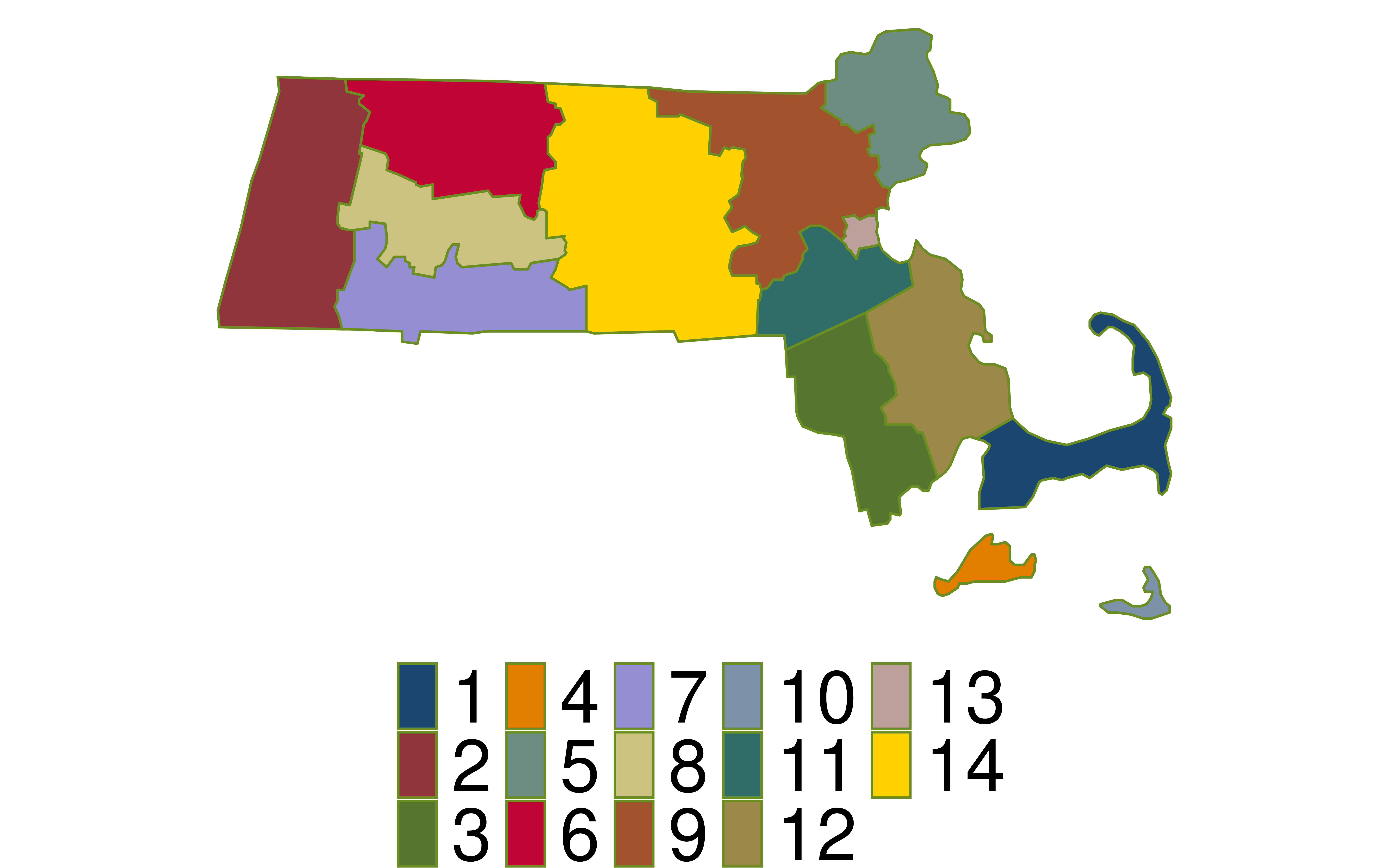
Are our clusters based on counties homogeneous?
Why is homogeneity important for cluster sampling?

FIA: Stratified Random Sampling

Break the landscape up into equally sized plots (~1 acre).
Put each plot in a stratum.
- For our example: stratum = county.
Take a simple random sample within every stratum.
- Don’t have to be equally sized!

# Do this for each stratum
sample(x = 1:---, size = ---)

Thoughts on this sampling design?

FIA: Systematic Random Sampling

This is FIA’s actual sampling design (okay, slightly simplified).

Break the landscape up into equally sized plots (~1 acre).
Number each plot from 1 to 6,755,200.
Use a random mechanism to pick starting point. Then sample about once every 6000 acres.

sample(x = 1:6755200, size = 1)

[1] 2845260

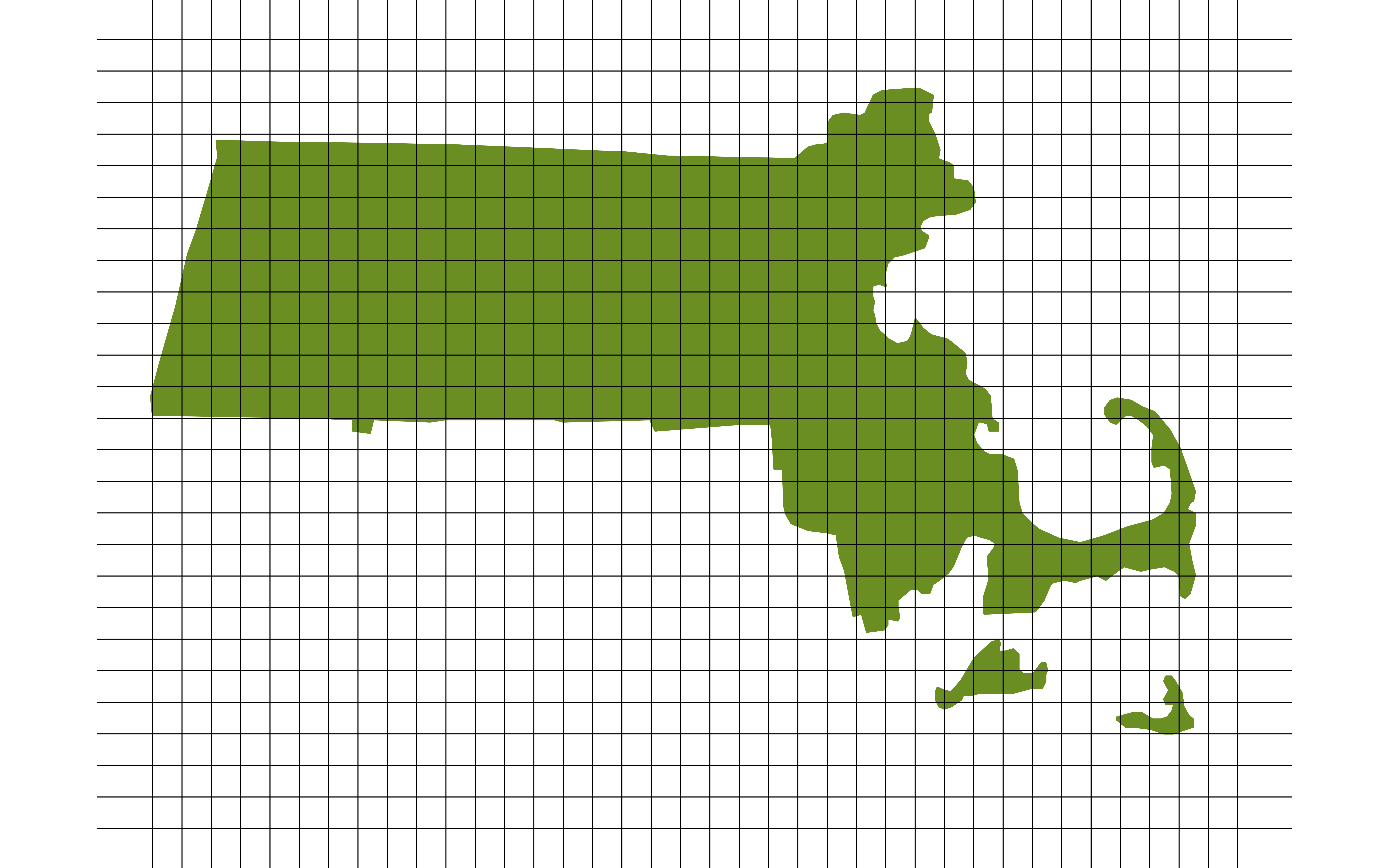
Why is this design better than simple random sampling?

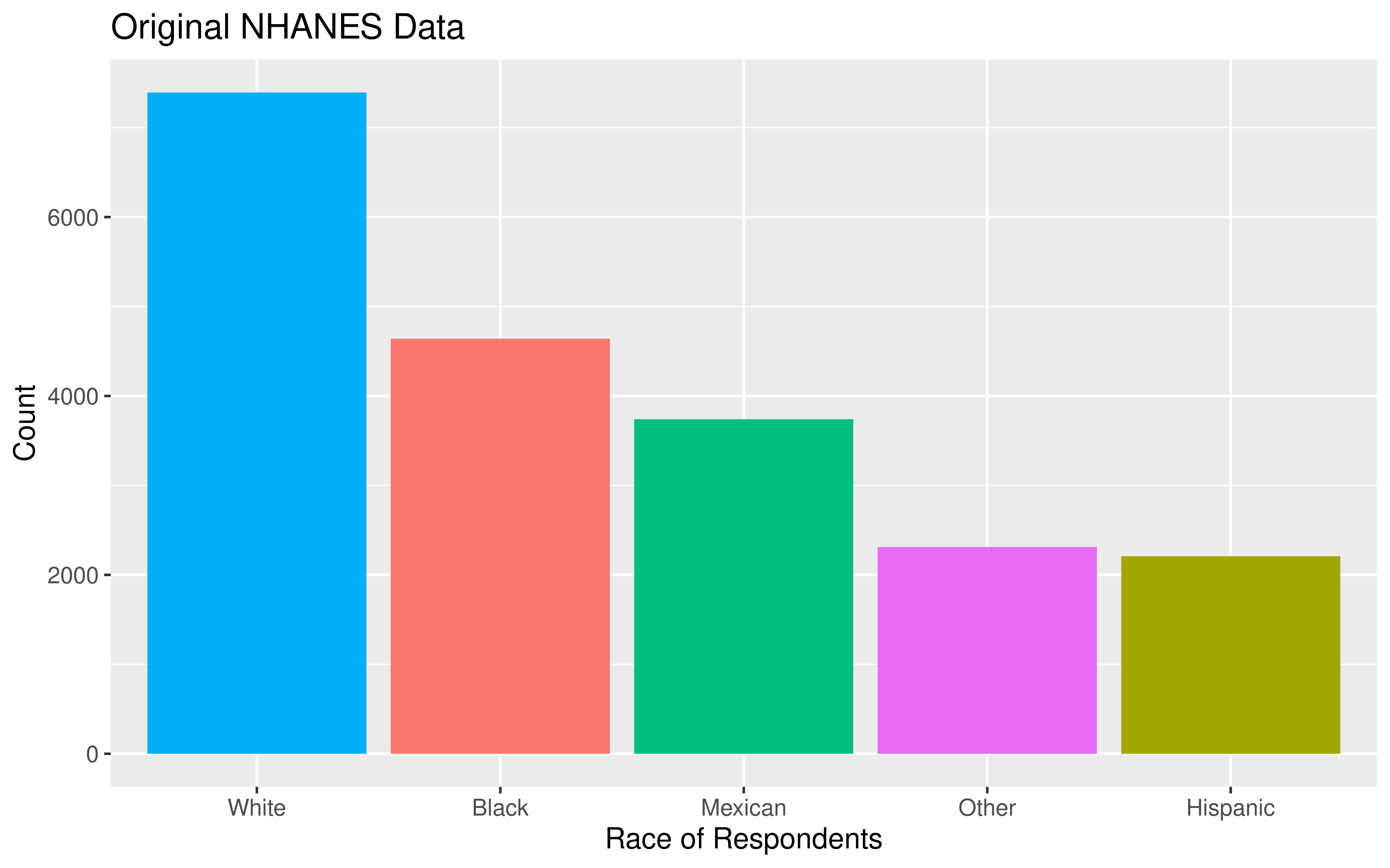
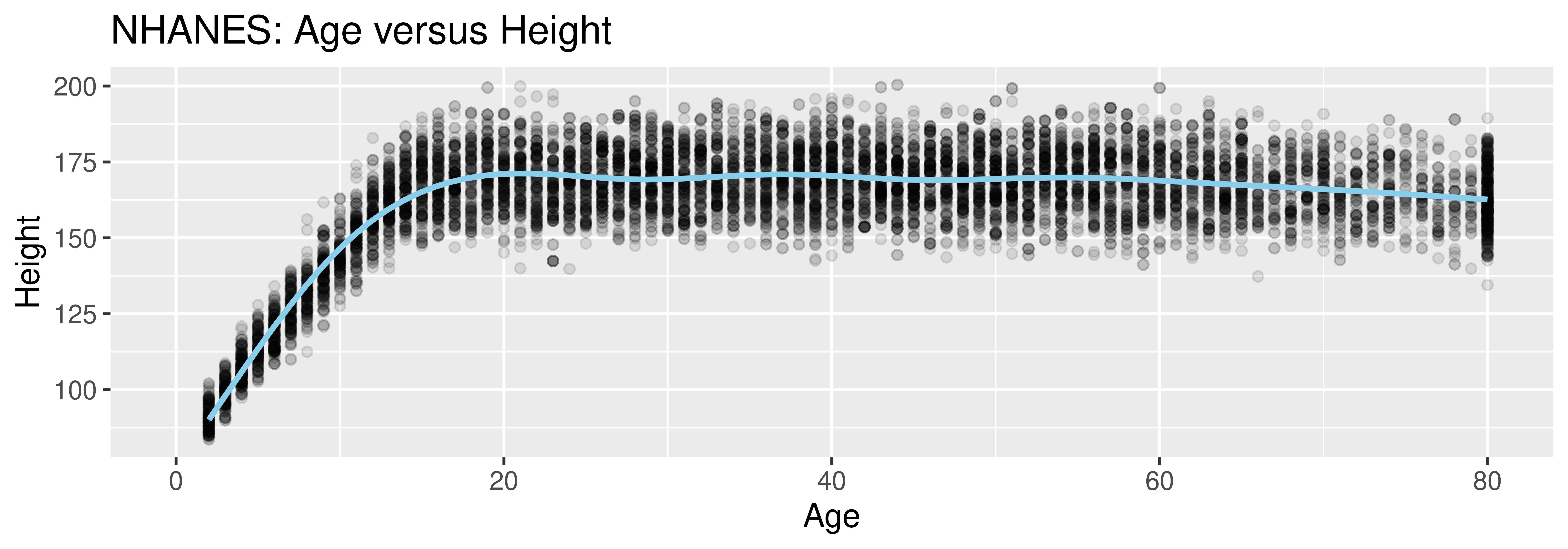
National Health and Nutrition Examination Survey

Mission: “Assess the health and nutritional status of adults and children in the United States.”

How are these data collected?

NHANES Sampling Design

Stage 1: US is stratified by geography and distribution of minority populations. Counties are randomly selected within each stratum.
Stage 2: From the sampled counties, city blocks are randomly selected. (City blocks are clusters.)
Stage 3: From sampled city blocks, households are randomly selected. (Households are clusters.)
Stage 4: From sampled households, people are randomly selected. For the sampled households, a mobile health vehicle goes to the house and medical professionals take the necessary measurements.

Why don’t they use simple random sampling?

Careful Using Non-Simple Random Sample Data

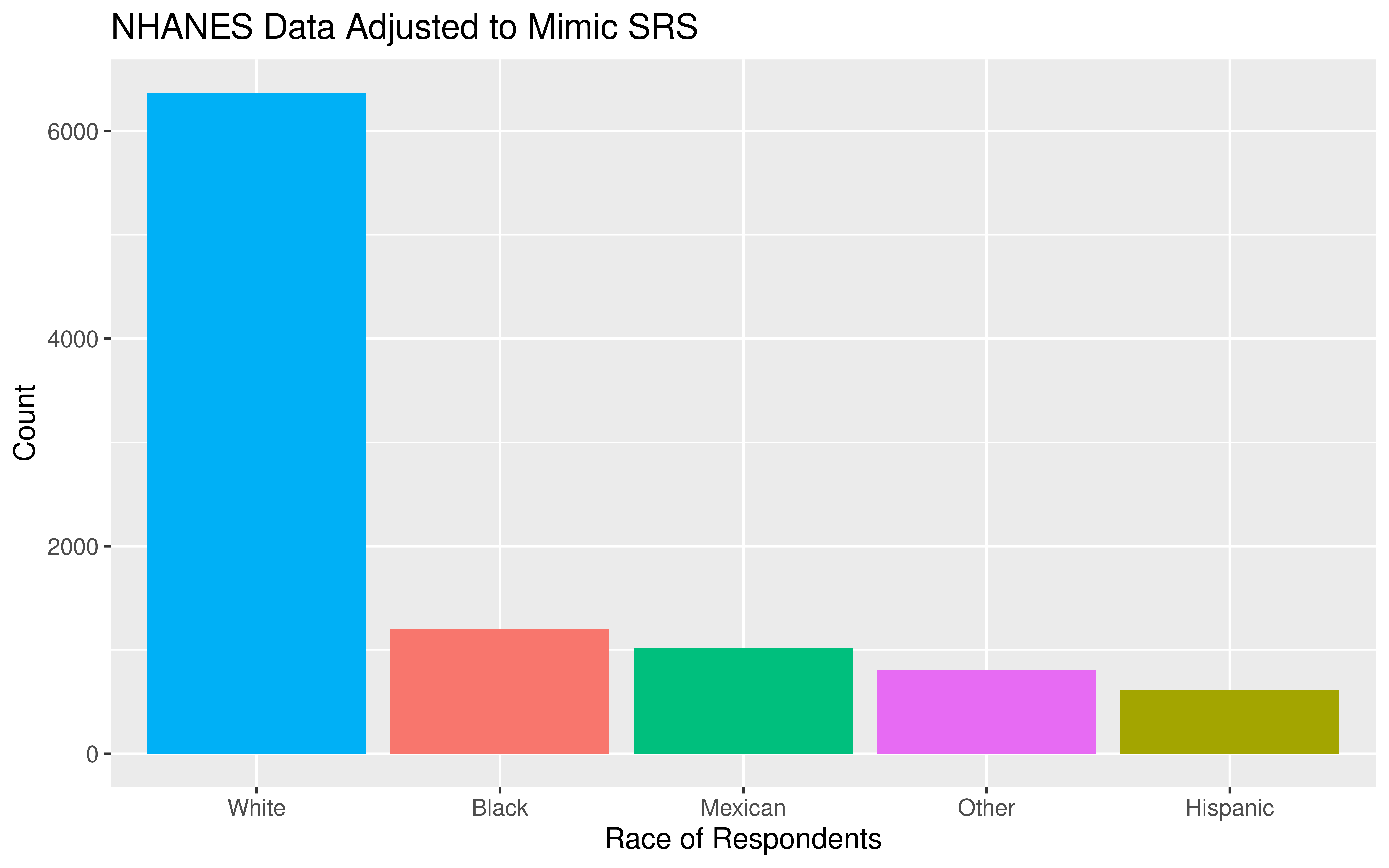
If you are dealing with data collected using a complex sampling design, I’d recommend taking an additional stats course, like Stat 160: Intro to Survey Sampling & Estimation!

Detour: Data Ethics

Data Ethics

“Good statistical practice is fundamentally based on transparent assumptions, reproducible results, and valid interpretations.” – Committee on Professional Ethics of the American Statistical Association (ASA)

The ASA has created “Ethical Guidelines for Statistical Practice”

→ These guidelines are for EVERYONE doing statistical work.

→ There are ethical decisions at all steps of the Data Analysis Process.

→ We will periodically refer to specific guidelines throughout this class.

“Above all, professionalism in statistical practice presumes the goal of advancing knowledge while avoiding harm; using statistics in pursuit of unethical ends is inherently unethical.”

Responsibilities to Research Subjects

“The ethical statistician protects and respects the rights and interests of human and animal subjects at all stages of their involvement in a project. This includes respondents to the census or to surveys, those whose data are contained in administrative records, and subjects of physically or psychologically invasive research.”

Responsibilities to Research Subjects

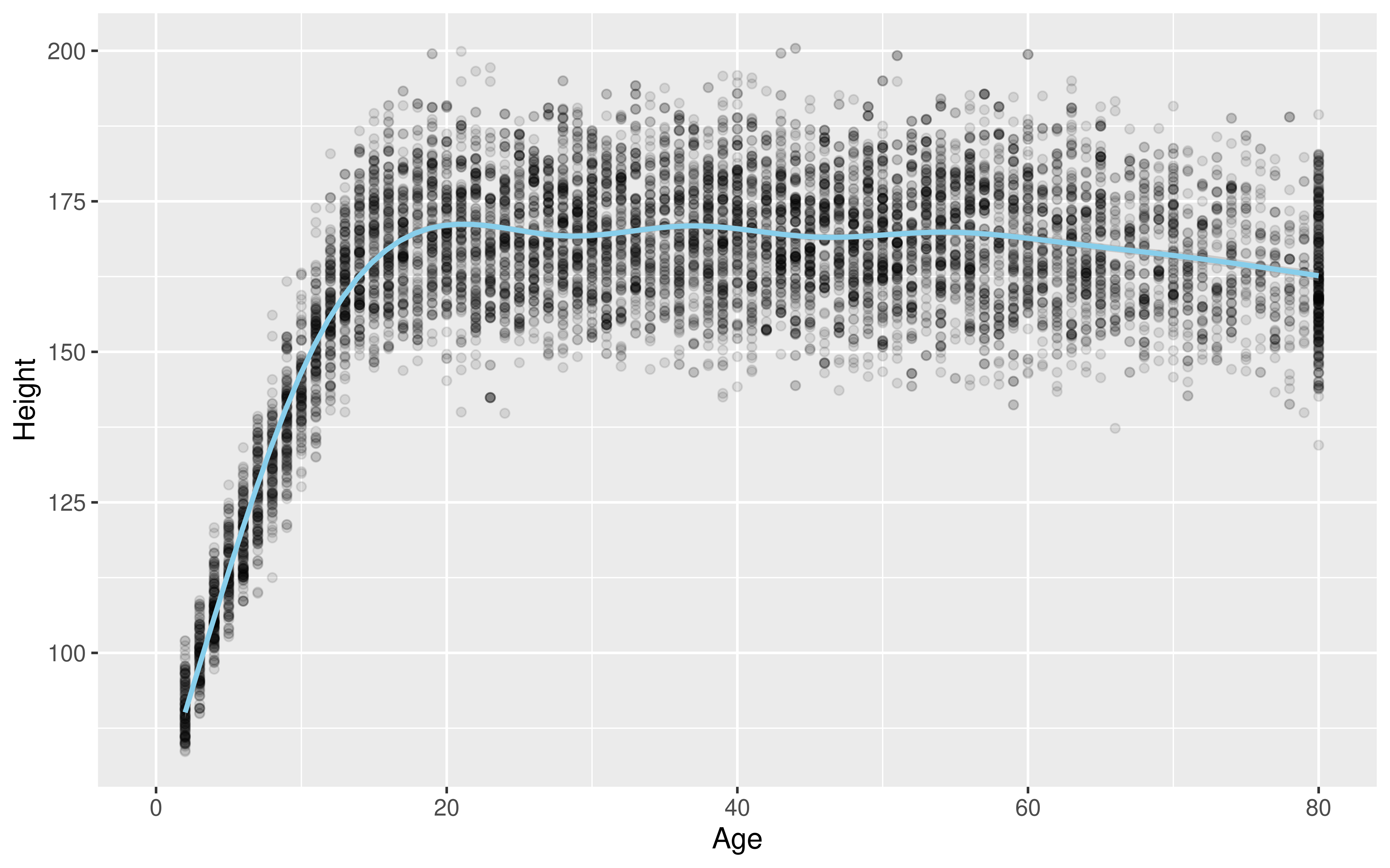
Why do you think the Age variable maxes out at 80?

“Protects the privacy and confidentiality of research subjects and data concerning them, whether obtained from the subjects directly, other persons, or existing records.”

Detour from Our Detour

library(tidyverse)
library(NHANES)

ggplot(data = NHANES, 
       mapping = aes(x = Age,
                     y = Height)) +
  geom_point(alpha = 0.1) +
  geom_smooth(color = "skyblue")

Detour from Our Detour

library(tidyverse)
library(NHANES)
library(emojifont)

NHANES <- mutate(NHANES, 
          heart = fontawesome("fa-heart"))

ggplot(data = NHANES, 
       mapping = aes(x = Age,
                     y = Height,
                     label = heart)) +
  geom_text(alpha = 0.1, color = "red",
            family='fontawesome-webfont',
            size = 16) +
  stat_smooth(color = "deeppink")

Announcements

Goals for Today

Getting Help with R

When to Get Help

When to Get Help

Which Are YOU?

Data Visualizer

Data Wrangler

Load Necessary Packages

Data Setting: Bureau of Labor Statistics (BLS) Consumer Expenditure Survey

CE Data

Smaller Sets of CE Data

Look at the Possible Joins

Joining Tips

Naming Wrangled Data

Live Coding

Sage Advice from ModernDive

Now for Data Collection

Motivating Our Discussion of Data Collection

Who are the data supposed to represent?

Who are the data supposed to represent?

Who are the data supposed to represent?

Who are the data supposed to represent?

Sampling Bias

Sampling Bias Example

Random Sampling

Types of random sampling

US Forest Inventory and Analysis Program

FIA: Simple Random Sampling

FIA: Cluster Random Sampling

FIA: Cluster Random Sampling

FIA: Cluster Random Sampling

FIA: Stratified Random Sampling

FIA: Systematic Random Sampling

National Health and Nutrition Examination Survey

NHANES Sampling Design

Careful Using Non-Simple Random Sample Data

Detour: Data Ethics

Data Ethics

Responsibilities to Research Subjects

Responsibilities to Research Subjects

Detour from Our Detour

Detour from Our Detour

Getting Help with `R`