Introduction to Modeling

Kelly McConville

Stat 100
Week 5 | Fall 2023

Announcements

• No lecture on Monday – University Holiday.
• Some Monday Office Hours will also be cancelled. Make sure to check the office hours schedule.
• Discuss upcoming exam:
  • Midterm next week
    • In-class: Wed, Oct 11th 10:30 - 11:45am
    • Oral: Wed afternoon - Fri, Oct 13th
    • No sections during midterm exam week!

Goals for Today

• Introduce statistical modeling

• Simple linear regression model

• Measuring correlation

Thoughts on Data Collection Goals

• Random assignment allows you to explore causal relationships between your explanatory variables and the predictor variables because the randomization makes the explanatory groups roughly similar.

• How do we draw causal conclusions from studies without random assignment?

  • With extreme care! Try to control for all possible confounding variables.
  • Discuss the associations/correlations you found. Use domain knowledge to address potentially causal links.
  • Take more stats to learn more about causal inference.

• But also consider the goals of your analysis. Often the research question isn’t causal.

Bottom Line: We often have to use imperfect data to make decisions.

Conclusions, Conclusions

Recap

Typical Analysis Goals

Descriptive: Want to estimate quantities related to the population.

→ How many trees are in Alaska?

Predictive: Want to predict the value of a variable.

→ Can I use remotely sensed data to predict forest types in Alaska?

Causal: Want to determine if changes in a variable cause changes in another variable.

→ Are insects causing the increased mortality rates for pinyon-juniper woodlands?

We will focus mainly on descriptive/causal modeling in this course. If you want to learn more about predictive modeling, take Stat 121A: Data Science 1 + Stat 121B: Data Science 2.

Form of the Model

\[ y = f(x) + \epsilon \]

Goal:

• Determine a reasonable form for \(f()\). (Ex: Line, curve, …)

• Estimate \(f()\) with \(\hat{f}()\) using the data.

• Generate predicted values: \(\hat y = \hat{f}(x)\).

Simple Linear Regression Model

Consider this model when:

• Response variable \((y)\): quantitative

• Explanatory variable \((x)\): quantitative

  • Have only ONE explanatory variable.

• AND, \(f()\) can be approximated by a line.

Example: The Ultimate Halloween Candy Power Ranking

“The social contract of Halloween is simple: Provide adequate treats to costumed masses, or be prepared for late-night tricks from those dissatisfied with your offer. To help you avoid that type of vengeance, and to help you make good decisions at the supermarket this weekend, we wanted to figure out what Halloween candy people most prefer. So we devised an experiment: Pit dozens of fun-sized candy varietals against one another, and let the wisdom of the crowd decide which one was best.” – Walt Hickey

“While we don’t know who exactly voted, we do know this: 8,371 different IP addresses voted on about 269,000 randomly generated matchups.2 So, not a scientific survey or anything, but a good sample of what candy people like.”

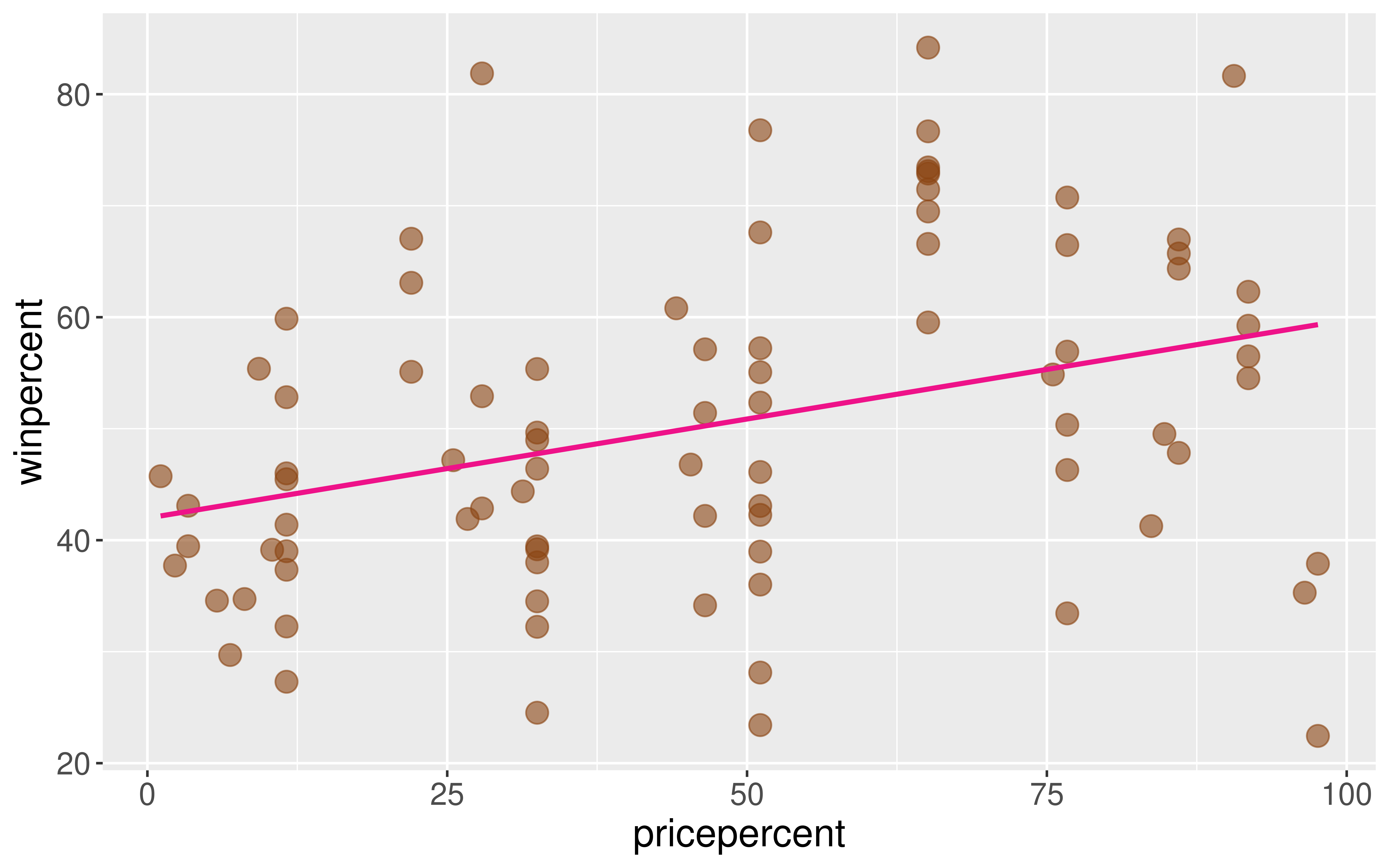
Example: The Ultimate Halloween Candy Power Ranking

Example: The Ultimate Halloween Candy Power Ranking

candy <- read_csv("https://raw.githubusercontent.com/fivethirtyeight/data/master/candy-power-ranking/candy-data.csv") %>%
  mutate(pricepercent = pricepercent*100)

glimpse(candy)

Rows: 85
Columns: 13
$ competitorname   <chr> "100 Grand", "3 Musketeers", "One dime", "One quarter…
$ chocolate        <dbl> 1, 1, 0, 0, 0, 1, 1, 0, 0, 0, 1, 0, 0, 0, 0, 0, 0, 0,…
$ fruity           <dbl> 0, 0, 0, 0, 1, 0, 0, 0, 0, 1, 0, 1, 1, 1, 1, 1, 1, 1,…
$ caramel          <dbl> 1, 0, 0, 0, 0, 0, 1, 0, 0, 1, 0, 0, 0, 0, 0, 0, 0, 0,…
$ peanutyalmondy   <dbl> 0, 0, 0, 0, 0, 1, 1, 1, 0, 0, 0, 0, 0, 0, 0, 0, 0, 0,…
$ nougat           <dbl> 0, 1, 0, 0, 0, 0, 1, 0, 0, 0, 1, 0, 0, 0, 0, 0, 0, 0,…
$ crispedricewafer <dbl> 1, 0, 0, 0, 0, 0, 0, 0, 0, 0, 0, 0, 0, 0, 0, 0, 0, 0,…
$ hard             <dbl> 0, 0, 0, 0, 0, 0, 0, 0, 0, 0, 0, 0, 0, 0, 1, 0, 1, 1,…
$ bar              <dbl> 1, 1, 0, 0, 0, 1, 1, 0, 0, 0, 1, 0, 0, 0, 0, 0, 0, 0,…
$ pluribus         <dbl> 0, 0, 0, 0, 0, 0, 0, 1, 1, 0, 0, 1, 1, 1, 0, 1, 0, 1,…
$ sugarpercent     <dbl> 0.732, 0.604, 0.011, 0.011, 0.906, 0.465, 0.604, 0.31…
$ pricepercent     <dbl> 86.0, 51.1, 11.6, 51.1, 51.1, 76.7, 76.7, 51.1, 32.5,…
$ winpercent       <dbl> 66.97173, 67.60294, 32.26109, 46.11650, 52.34146, 50.…

Example: The Ultimate Halloween Candy Power Ranking

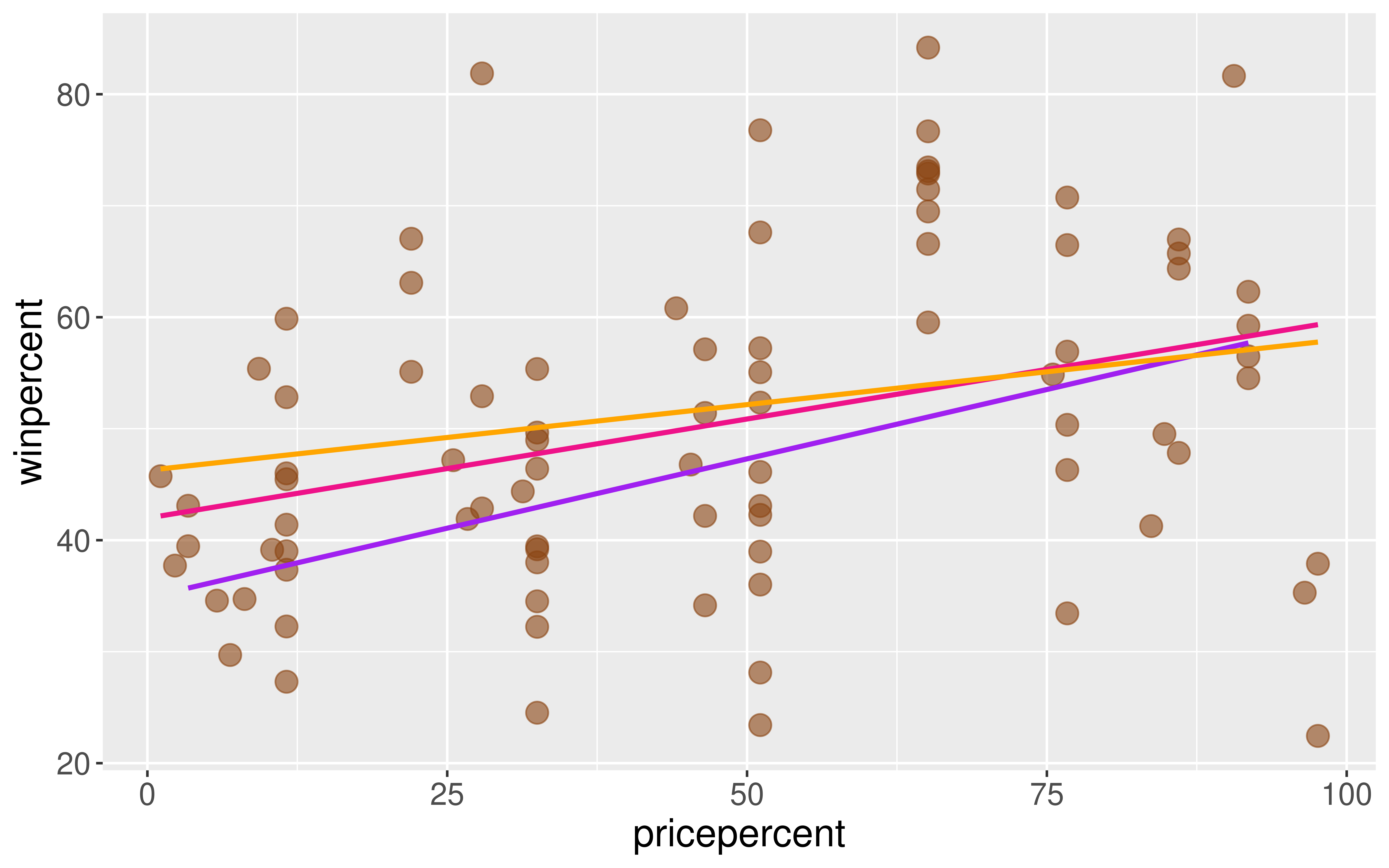
• Linear trend?

• Direction of trend?

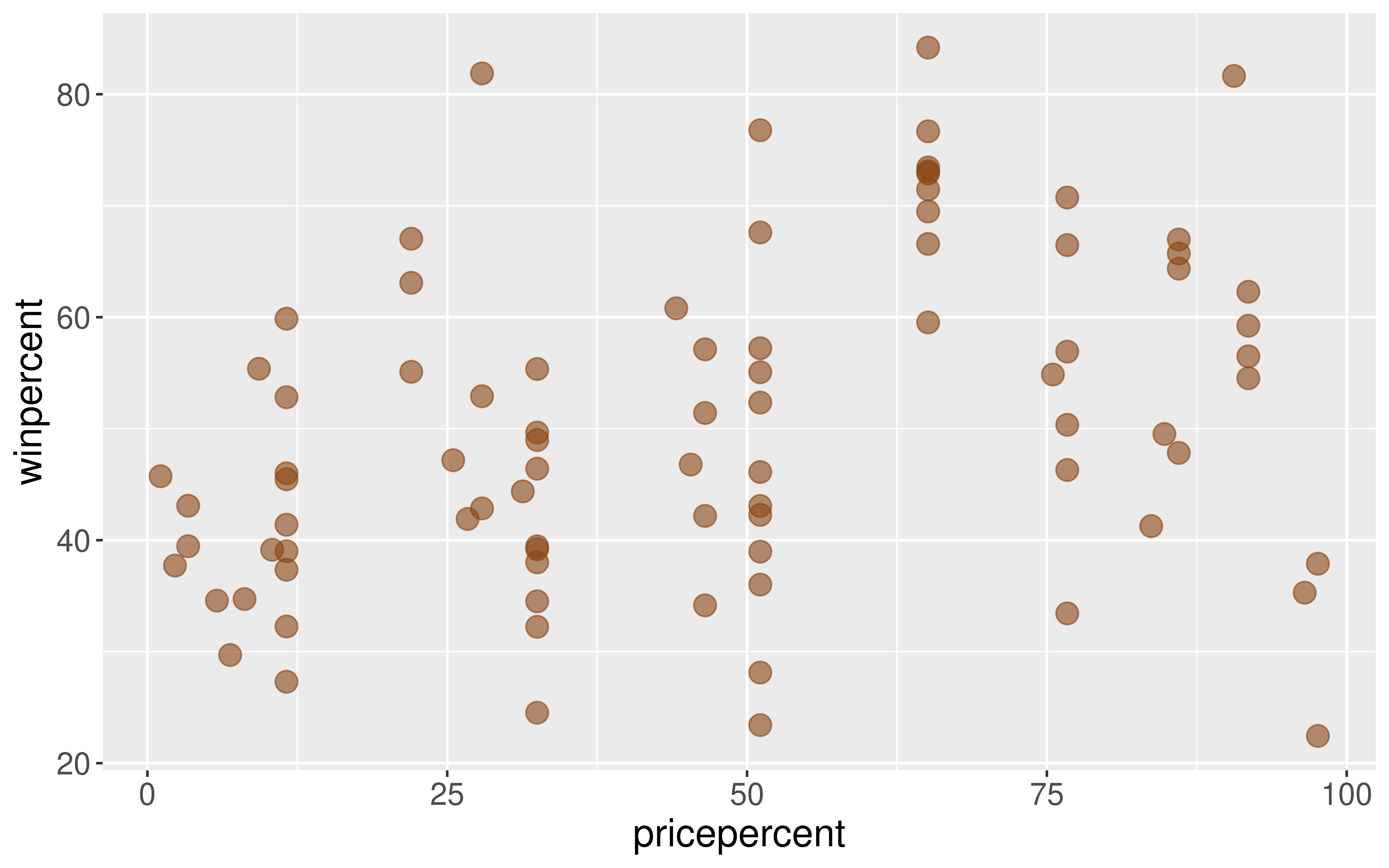
Example: The Ultimate Halloween Candy Power Ranking

• A simple linear regression model would be suitable for these data.

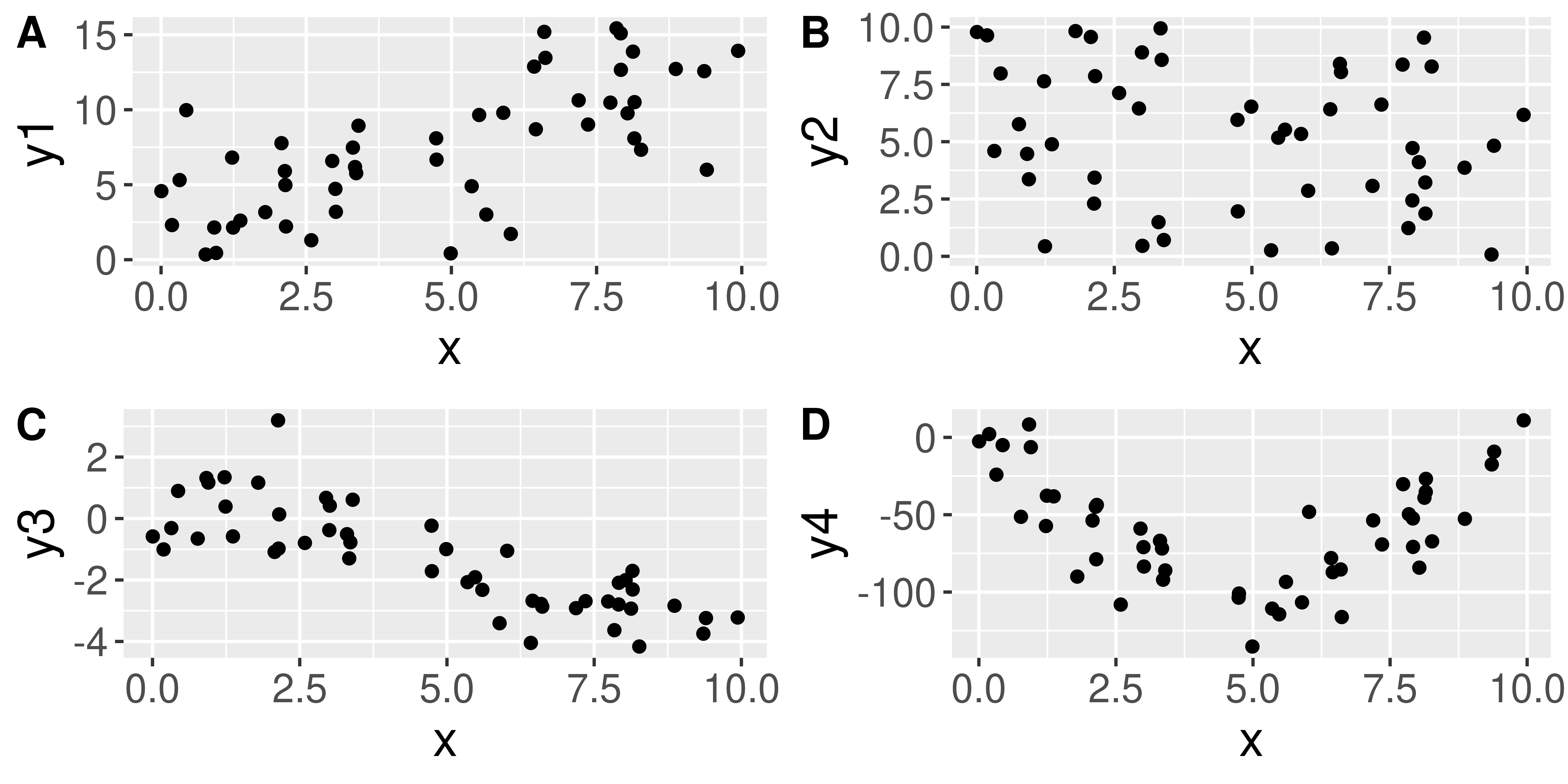
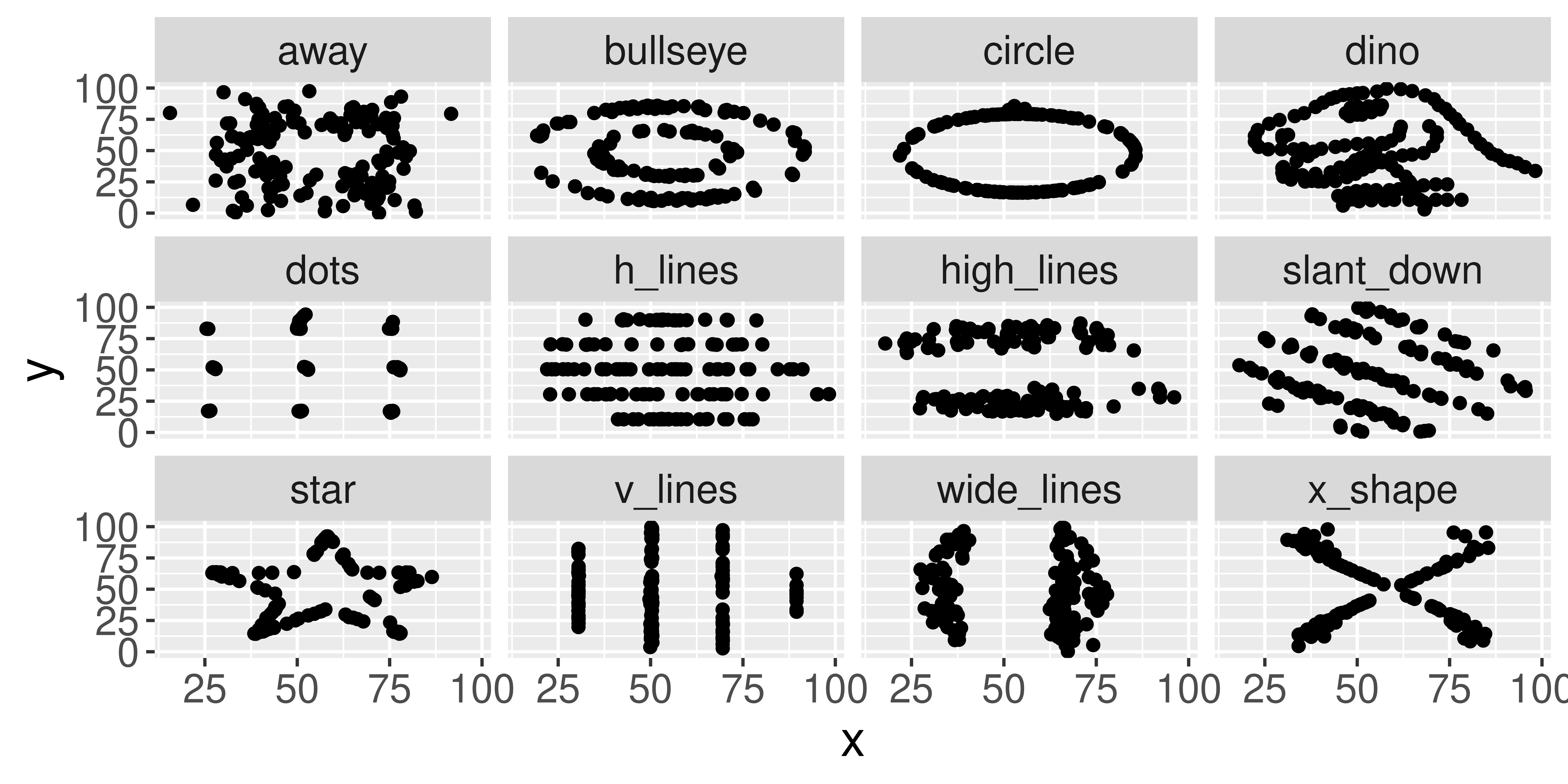
• But first, let’s describe more plots!

• Need a summary statistics that quantifies the strength and relationship of the linear trend!

(Sample) Correlation Coefficient

• Measures the strength and direction of linear relationship between two quantitative variables

• Symbol: \(r\)

• Always between -1 and 1

• Sign indicates the direction of the relationship

• Magnitude indicates the strength of the linear relationship

candy %>%
  summarize(cor = cor(pricepercent, winpercent))

# A tibble: 1 × 1
    cor
  <dbl>
1 0.345

Any guesses on the correlations for A, B, C, or D?

dat %>%
  summarize(A = cor(x, y1), B = cor(x, y2),
            C = cor(x, y3), D = cor(x, y4))

# A tibble: 1 × 4
      A      B      C      D
  <dbl>  <dbl>  <dbl>  <dbl>
1 0.695 -0.217 -0.815 -0.113

New Example

# Correlation coefficients
dat2 %>%
  group_by(dataset) %>%
  summarize(cor = cor(x, y))

# A tibble: 12 × 2
   dataset        cor
   <chr>        <dbl>
 1 away       -0.0641
 2 bullseye   -0.0686
 3 circle     -0.0683
 4 dino       -0.0645
 5 dots       -0.0603
 6 h_lines    -0.0617
 7 high_lines -0.0685
 8 slant_down -0.0690
 9 star       -0.0630
10 v_lines    -0.0694
11 wide_lines -0.0666
12 x_shape    -0.0656

• Conclude that \(x\) and \(y\) have the same relationship across these different datasets because the correlation is the same?

Always graph the data when exploring relationships!

Returning to the Simple Linear Regression model…

Simple Linear Regression

Let’s return to the Candy Example.

• A line is a reasonable model form.

• Where should the line be?

  • Slope? Intercept?

Form of the SLR Model

\[ \begin{align} y &= f(x) + \epsilon \\ y &= \beta_o + \beta_1 x + \epsilon \end{align} \]

• Need to determine the best estimates of \(\beta_o\) and \(\beta_1\).

Distinguishing between the population and the sample

\[ y = \beta_o + \beta_1 x + \epsilon \]

• Parameters:
  • Based on the population
  • Unknown then if don’t have data on the whole population
  • EX: \(\beta_o\) and \(\beta_1\)

\[ \hat{y} = \hat{ \beta}_o + \hat{\beta}_1 x \]

• Statistics:
  • Based on the sample data
  • Known
  • Usually estimate a population parameter
  • EX: \(\hat{\beta}_o\) and \(\hat{\beta}_1\)

Method of Least Squares

Need two key definitions:

• Fitted value: The estimated value of the \(i\)-th case

\[ \hat{y}_i = \hat{\beta}_o + \hat{\beta}_1 x_i \]

• Residuals: The observed error term for the \(i\)-th case

\[ e_i = y_i - \hat{y}_i \]

Goal: Pick values for \(\hat{\beta}_o\) and \(\hat{\beta}_1\) so that the residuals are small!

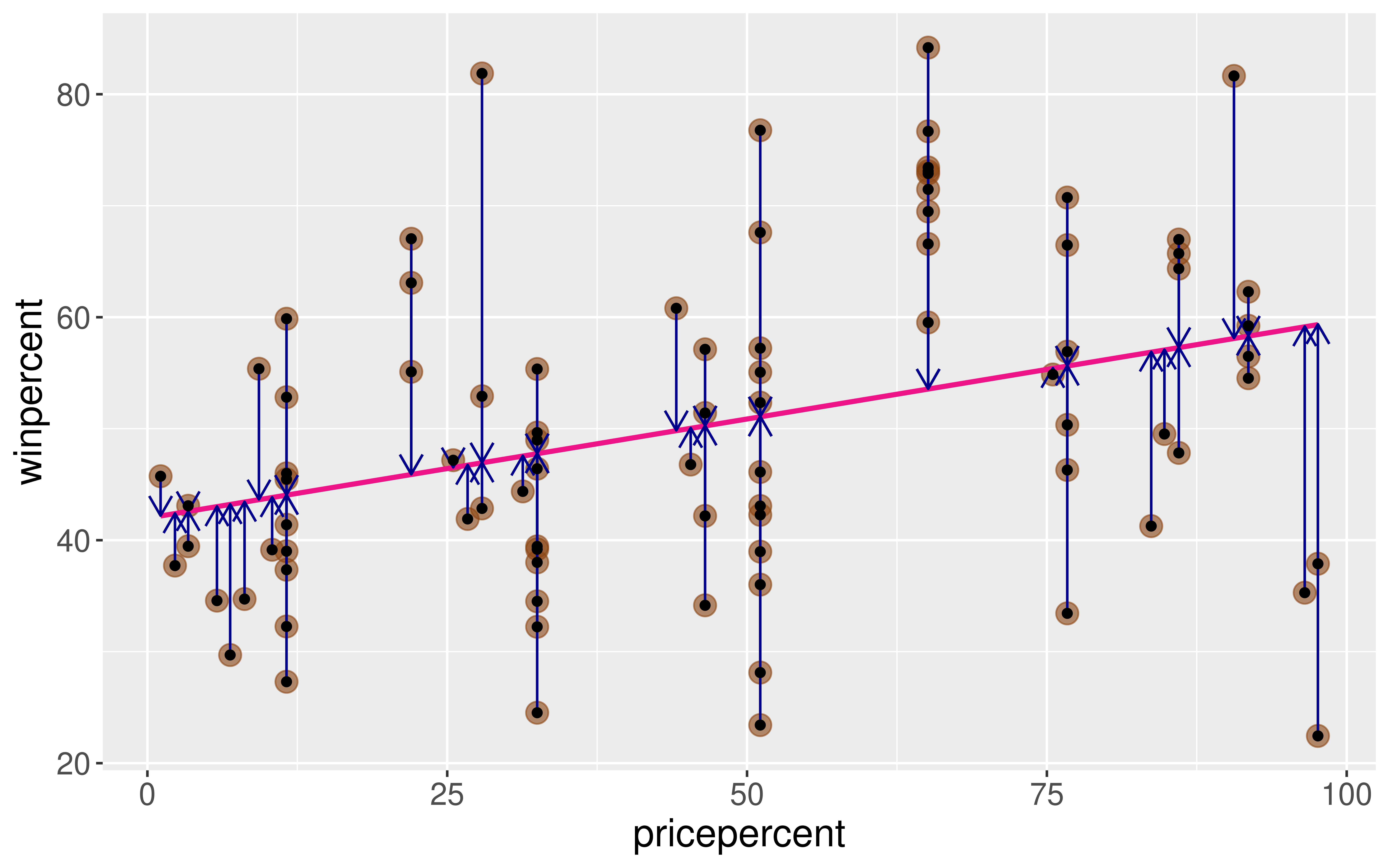
Method of Least Squares

• Want residuals to be small.

• Minimize a function of the residuals.

• Minimize:

\[ \sum_{i = 1}^n e^2_i \]

Method of Least Squares

After minimizing the sum of squared residuals, you get the following equations:

Get the following equations:

\[ \begin{align} \hat{\beta}_1 &= \frac{ \sum_{i = 1}^n (x_i - \bar{x}) (y_i - \bar{y})}{ \sum_{i = 1}^n (x_i - \bar{x})^2} \\ \hat{\beta}_o &= \bar{y} - \hat{\beta}_1 \bar{x} \end{align} \] where

\[ \begin{align} \bar{y} = \frac{1}{n} \sum_{i = 1}^n y_i \quad \mbox{and} \quad \bar{x} = \frac{1}{n} \sum_{i = 1}^n x_i \end{align} \]

Method of Least Squares

Then we can estimate the whole function with:

\[ \hat{y} = \hat{\beta}_o + \hat{\beta}_1 x \]

Called the least squares line or the line of best fit.

Method of Least Squares

ggplot2 will compute the line and add it to your plot using geom_smooth(method = "lm")

ggplot(data = candy, 
       mapping = aes(x = pricepercent,
                     y = winpercent)) +
  geom_point(alpha = 0.6, size = 4, 
             color = "chocolate4") +
  geom_smooth(method = "lm", se = FALSE,
              color = "deeppink2")

But what are the exact values of \(\hat{\beta}_o\) and \(\hat{\beta}_1\)?

Constructing the Simple Linear Regression Model in R

mod <- lm(winpercent ~ pricepercent, data = candy)

library(moderndive)
get_regression_table(mod)

# A tibble: 2 × 7
  term         estimate std_error statistic p_value lower_ci upper_ci
  <chr>           <dbl>     <dbl>     <dbl>   <dbl>    <dbl>    <dbl>
1 intercept      42.0       2.91      14.4    0       36.2     47.8  
2 pricepercent    0.178     0.053      3.35   0.001    0.072    0.283

• Interpretation of the coefficients?

Prediction

new_cases <- data.frame(pricepercent = c(25, 85, 150))
predict(mod, newdata = new_cases)

       1        2        3 
46.42443 57.09409 68.65289 

• We didn’t have any treats in our sample with a price percentage of 85%. Can we still make this prediction?
  • Called interpolation

• We didn’t have any treats in our sample with a price percentage of 150%. Can we still make this prediction?
  • Called extrapolation

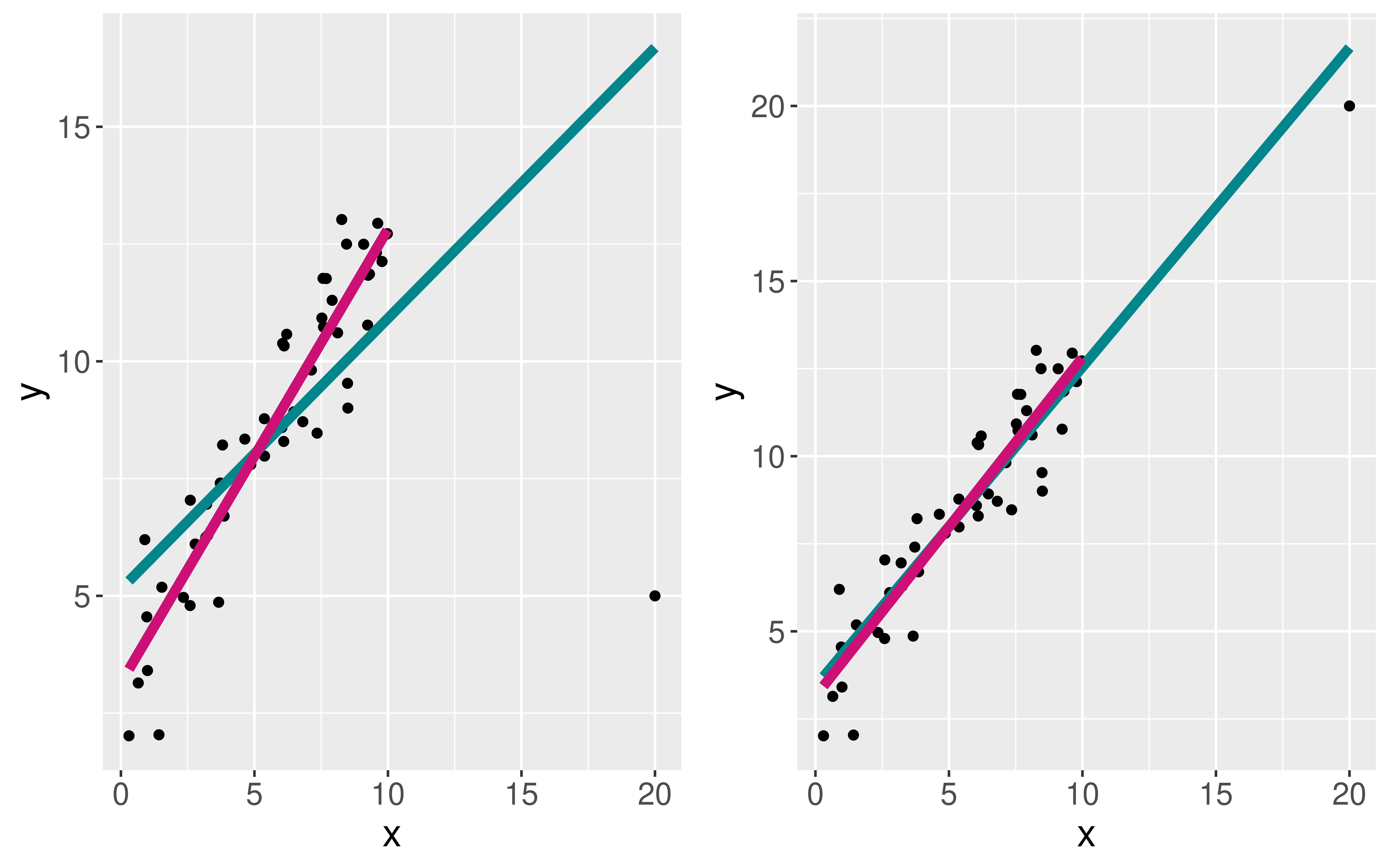
Cautions

• Careful to only predict values within the range of \(x\) values in the sample.

• Make sure to investigate outliers: observations that fall far from the cloud of points.

Reminders

• No lecture on Monday – University Holiday.
• Some Monday Office Hours will also be cancelled. Make sure to check the office hours schedule.
• Midterm next week
  • In-class: Wed, Oct 11th 10:30 - 11:45am
  • Oral: Wed afternoon - Fri, Oct 13th
• No sections during midterm exam week!