Multiple Linear Regression

Kelly McConville

Stat 100
Week 7 | Fall 2023

Announcements

• This Wednesday we will be in Sanders Hall instead of Hall C.
• Back to a normal schedule.
  • Have section & wrap-ups this week!
• Notes on the midterm.

Goals for Today

• Recap: Simple linear regression model
• Broadening our idea of linear regression

• Regression with a single, categorical explanatory variable
• Regression with multiple explanatory variables

Simple Linear Regression

Consider this model when:

• Response variable \((y)\): quantitative

• Explanatory variable \((x)\): quantitative

  • Have only ONE explanatory variable.

• AND, \(f()\) can be approximated by a line:

\[ \begin{align} y &= \beta_o + \beta_1 x + \epsilon \end{align} \]

Cautions

• Careful to only predict values within the range of \(x\) values in the sample.

• Make sure to investigate outliers: observations that fall far from the cloud of points.

Linear Regression

Linear regression is a flexible class of models that allow for:

• Both quantitative and categorical explanatory variables.

• Multiple explanatory variables.

• Curved relationships between the response variable and the explanatory variable.

• BUT the response variable is quantitative.

What About A Categorical Explanatory Variable?

• Response variable \((y)\): quantitative

• Have 1 categorical explanatory variable \((x)\) with two categories.

• Model form:

\[ \begin{align} y &= \beta_o + \beta_1 x + \epsilon \end{align} \]

• First, need to convert the categories of \(x\) to numbers.

Example: Halloween Candy

candy <- read_csv("https://raw.githubusercontent.com/fivethirtyeight/data/master/candy-power-ranking/candy-data.csv")
glimpse(candy)

Rows: 85
Columns: 13
$ competitorname   <chr> "100 Grand", "3 Musketeers", "One dime", "One quarter…
$ chocolate        <dbl> 1, 1, 0, 0, 0, 1, 1, 0, 0, 0, 1, 0, 0, 0, 0, 0, 0, 0,…
$ fruity           <dbl> 0, 0, 0, 0, 1, 0, 0, 0, 0, 1, 0, 1, 1, 1, 1, 1, 1, 1,…
$ caramel          <dbl> 1, 0, 0, 0, 0, 0, 1, 0, 0, 1, 0, 0, 0, 0, 0, 0, 0, 0,…
$ peanutyalmondy   <dbl> 0, 0, 0, 0, 0, 1, 1, 1, 0, 0, 0, 0, 0, 0, 0, 0, 0, 0,…
$ nougat           <dbl> 0, 1, 0, 0, 0, 0, 1, 0, 0, 0, 1, 0, 0, 0, 0, 0, 0, 0,…
$ crispedricewafer <dbl> 1, 0, 0, 0, 0, 0, 0, 0, 0, 0, 0, 0, 0, 0, 0, 0, 0, 0,…
$ hard             <dbl> 0, 0, 0, 0, 0, 0, 0, 0, 0, 0, 0, 0, 0, 0, 1, 0, 1, 1,…
$ bar              <dbl> 1, 1, 0, 0, 0, 1, 1, 0, 0, 0, 1, 0, 0, 0, 0, 0, 0, 0,…
$ pluribus         <dbl> 0, 0, 0, 0, 0, 0, 0, 1, 1, 0, 0, 1, 1, 1, 0, 1, 0, 1,…
$ sugarpercent     <dbl> 0.732, 0.604, 0.011, 0.011, 0.906, 0.465, 0.604, 0.31…
$ pricepercent     <dbl> 0.860, 0.511, 0.116, 0.511, 0.511, 0.767, 0.767, 0.51…
$ winpercent       <dbl> 66.97173, 67.60294, 32.26109, 46.11650, 52.34146, 50.…

What might be a good categorical explanatory variable of winpercent?

Exploratory Data Analysis

Before building the model, let’s explore and visualize the data!

• What dplyr functions should I use to find the mean and sd of winpercent by the categories of chocolate?

• What graph should we use to visualize the winpercent scores by chocolate?

Exploratory Data Analysis

# Summarize
candy %>%
  group_by(chocolate) %>%
  summarize(count = n(), mean_win = mean(winpercent), 
            sd_win = sd(winpercent))

# A tibble: 2 × 4
  chocolate count mean_win sd_win
      <dbl> <int>    <dbl>  <dbl>
1         0    48     42.1   10.2
2         1    37     60.9   12.8

Exploratory Data Analysis

ggplot(candy, aes(x = factor(chocolate), 
                   y = winpercent, 
                  fill = factor(chocolate))) +
  geom_boxplot() +
    stat_summary(fun = mean,
                 geom = "point",
                 color = "yellow",
                 size = 4) +
  guides(fill = "none") +
  scale_fill_manual(values =
                      c("0" = "deeppink",
                        "1" = "chocolate4")) +
  scale_x_discrete(labels = c("No", "Yes"),
                   name =
          "Does the candy contain chocolate?")

Fit the Linear Regression Model

Model Form:

\[ \begin{align} y &= \beta_o + \beta_1 x + \epsilon \end{align} \]

When \(x = 0\):

When \(x = 1\):

mod <- lm(winpercent ~ chocolate, data = candy)
library(moderndive)
get_regression_table(mod)

# A tibble: 2 × 7
  term      estimate std_error statistic p_value lower_ci upper_ci
  <chr>        <dbl>     <dbl>     <dbl>   <dbl>    <dbl>    <dbl>
1 intercept     42.1      1.65     25.6        0     38.9     45.4
2 chocolate     18.8      2.50      7.52       0     13.8     23.7

Notes

• When the explanatory variable is categorical, \(\beta_o\) and \(\beta_1\) no longer represent the intercept and slope.

• Now \(\beta_o\) represents the (population) mean of the response variable when \(x = 0\).

• And, \(\beta_1\) represents the change in the (population) mean response going from \(x = 0\) to \(x = 1\).

• Can also do prediction:

new_candy <- data.frame(chocolate = c(0, 1))
predict(mod, newdata = new_candy)

       1        2 
42.14226 60.92153 

Turns Out Reese’s Miniatures Are Under-Priced…

Multiple Linear Regression

Form of the Model:

\[ \begin{align} y &= \beta_o + \beta_1 x_1 + \beta_2 x_2 + \cdots + \beta_p x_p + \epsilon \end{align} \]

How does extending to more predictors change our process?

• What doesn’t change:
  • Still use Method of Least Squares to estimate coefficients
  • Still use lm() to fit the model and predict() for prediction
• What does change:
  • Meaning of the coefficients are more complicated and depend on other variables in the model
  • Need to decide which variables to include and how (linear term, squared term…)

Multiple Linear Regression

• We are going to see a few examples of multiple linear regression today and next lecture.

• We will need to return to modeling later in the course to more definitively answer questions about model selection.

Example

Meadowfoam is a plant that grows in the Pacific Northwest and is harvested for its seed oil. In a randomized experiment, researchers at Oregon State University looked at how two light-related factors influenced the number of flowers per meadowfoam plant, the primary measure of productivity for this plant. The two light measures were light intensity (in mmol/ \(m^2\) /sec) and the timing of onset of the light (early or late in terms of photo periodic floral induction).

Response variable:

Explanatory variables:

Model Form:

Data Loading and Wrangling

library(tidyverse)
library(Sleuth3)
data(case0901)

# Recode the timing variable
count(case0901, Time)

  Time  n
1    1 12
2    2 12

case0901 <- case0901 %>%
  mutate(TimeCat = case_when(
    Time == 1 ~ "Late",
    Time == 2 ~ "Early"
    )) 
count(case0901, TimeCat)

  TimeCat  n
1   Early 12
2    Late 12

Visualizing the Data

ggplot(case0901,
       aes(x = Intensity,
           y = Flowers,
           color = TimeCat)) + 
  geom_point(size = 4)

Why don’t I have to include data = and mapping = in my ggplot() layer?

Building the Linear Regression Model

Full model form:

modFlowers <- lm(Flowers ~ Intensity + TimeCat, data = case0901)

library(moderndive)
get_regression_table(modFlowers)

# A tibble: 3 × 7
  term          estimate std_error statistic p_value lower_ci upper_ci
  <chr>            <dbl>     <dbl>     <dbl>   <dbl>    <dbl>    <dbl>
1 intercept        83.5      3.27      25.5        0   76.7      90.3 
2 Intensity        -0.04     0.005     -7.89       0   -0.051    -0.03
3 TimeCat: Late   -12.2      2.63      -4.62       0  -17.6      -6.69

• Estimated regression line for \(x_2 = 1\):

• Estimated regression line for \(x_2 = 0\):

Appropriateness of Model Form

ggplot(case0901, 
       aes(x = Intensity,
           y = Flowers,
           color = TimeCat)) + 
  geom_point(size = 4) + 
  geom_smooth(method = "lm", se = FALSE)

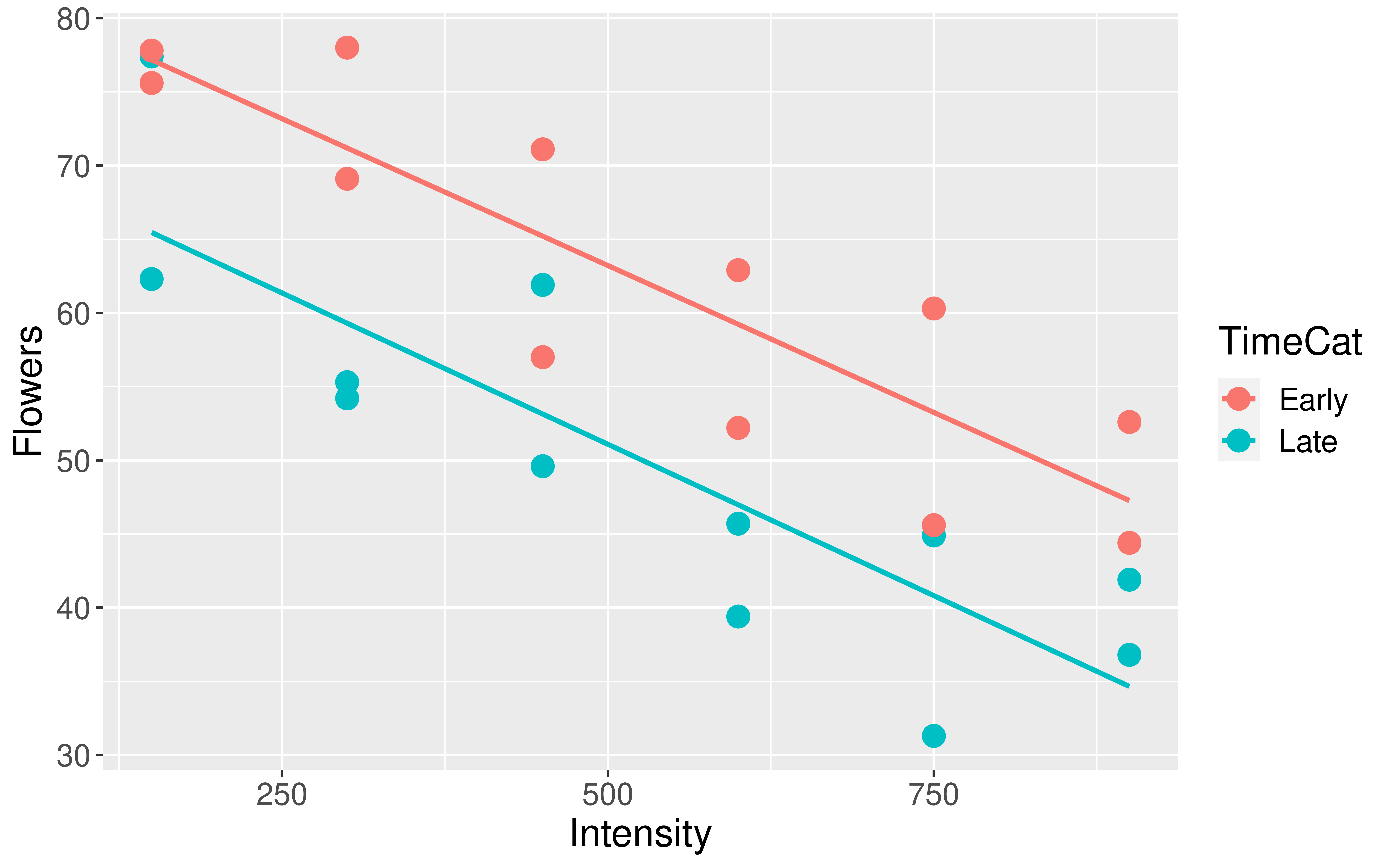
Is the assumption of equal slopes reasonable here?

Prediction

flowersNew <- data.frame(Intensity = c(700, 700), TimeCat = c("Early", "Late"))
flowersNew

  Intensity TimeCat
1       700   Early
2       700    Late

predict(modFlowers, newdata = flowersNew)

       1        2 
55.13417 42.97583 

New Example

For this example, we will use data collected by the website pollster.com, which aggregated 102 presidential polls from August 29th, 2008 through the end of September. We want to determine the best model to explain the variable Margin, measured by the difference in preference between Barack Obama and John McCain. Our potential predictors are Days (the number of days after the Democratic Convention) and Charlie (indicator variable on whether poll was conducted before or after the first ABC interview of Sarah Palin with Charlie Gibson).

library(Stat2Data)
data("Pollster08")
glimpse(Pollster08)

Rows: 102
Columns: 11
$ PollTaker <fct> Rasmussen, Zogby, Diageo/Hotline, CBS, CNN, Rasmussen, ARG, …
$ PollDates <fct> 8/28-30/08, 8/29-30/08, 8/29-31/08, 8/29-31/08, 8/29-31/08, …
$ MidDate   <fct> 8/29, 8/30, 8/30, 8/30, 8/30, 8/31, 8/31, 9/1, 9/2, 9/2, 9/2…
$ Days      <int> 1, 2, 2, 2, 2, 3, 3, 4, 5, 5, 5, 5, 6, 6, 8, 8, 9, 9, 9, 9, …
$ n         <int> 3000, 2020, 805, 781, 927, 3000, 1200, 1728, 2771, 1000, 734…
$ Pop       <fct> LV, LV, RV, RV, RV, LV, LV, RV, RV, A, RV, LV, LV, RV, RV, R…
$ McCain    <int> 46, 47, 39, 40, 48, 45, 43, 36, 42, 39, 42, 44, 46, 40, 48, …
$ Obama     <int> 49, 45, 48, 48, 49, 51, 49, 40, 49, 42, 42, 49, 48, 46, 45, …
$ Margin    <int> 3, -2, 9, 8, 1, 6, 6, 4, 7, 3, 0, 5, 2, 6, -3, 5, -4, -1, -2…
$ Charlie   <int> 0, 0, 0, 0, 0, 0, 0, 0, 0, 0, 0, 0, 0, 0, 0, 0, 0, 0, 0, 0, …
$ Meltdown  <int> 0, 0, 0, 0, 0, 0, 0, 0, 0, 0, 0, 0, 0, 0, 0, 0, 0, 0, 0, 0, …

Response variable:

Explanatory variables:

Visualizing the Data

ggplot(Pollster08,
       aes(x = Days,
           y = Margin, 
           color = Charlie)) +
  geom_point(size = 3)

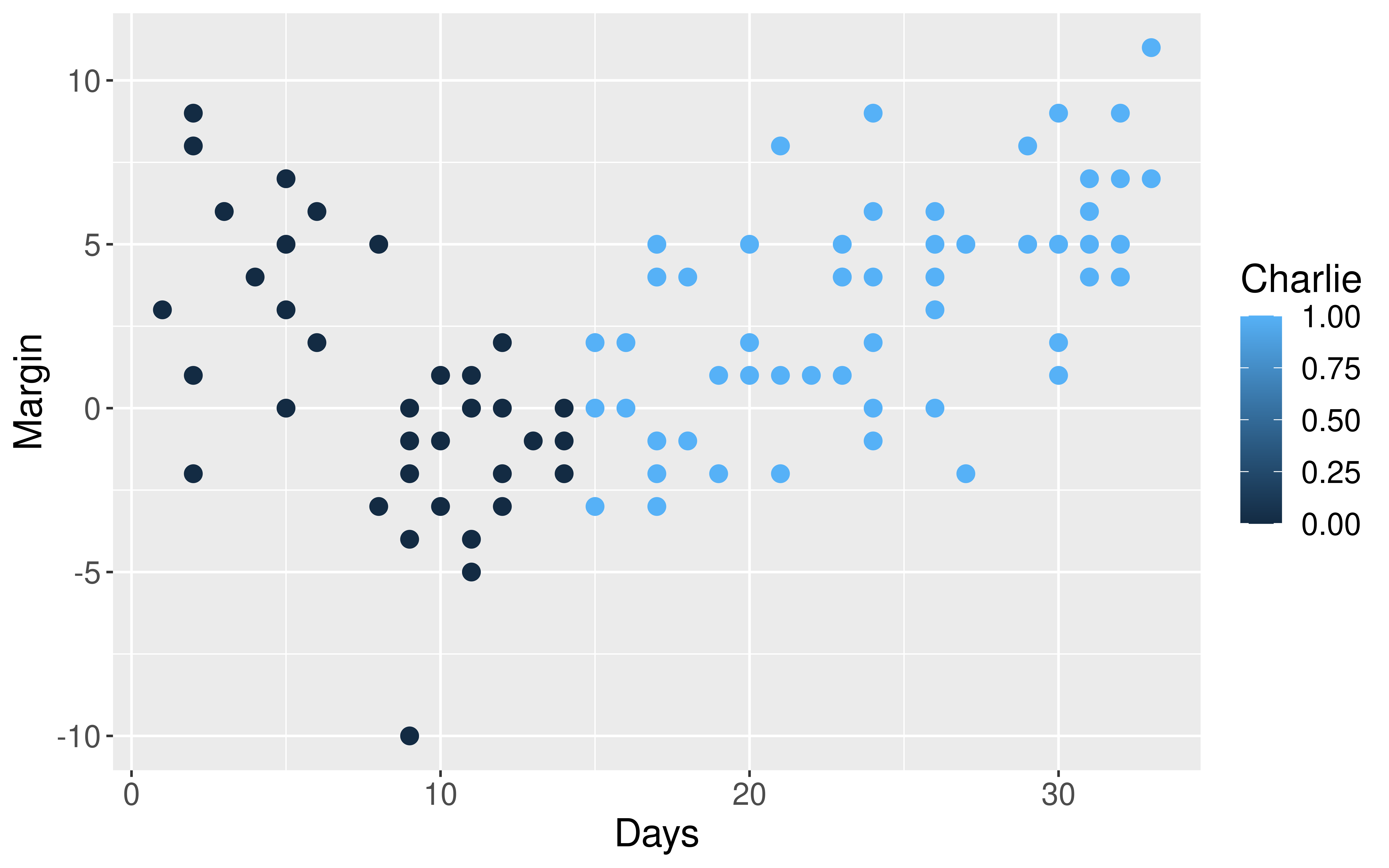
What is wrong with how one of the variables is mapped in the graph?

Visualizing the Data

ggplot(Pollster08,
       aes(x = Days,
           y = Margin, 
           color = factor(Charlie))) +
  geom_point(size = 3)

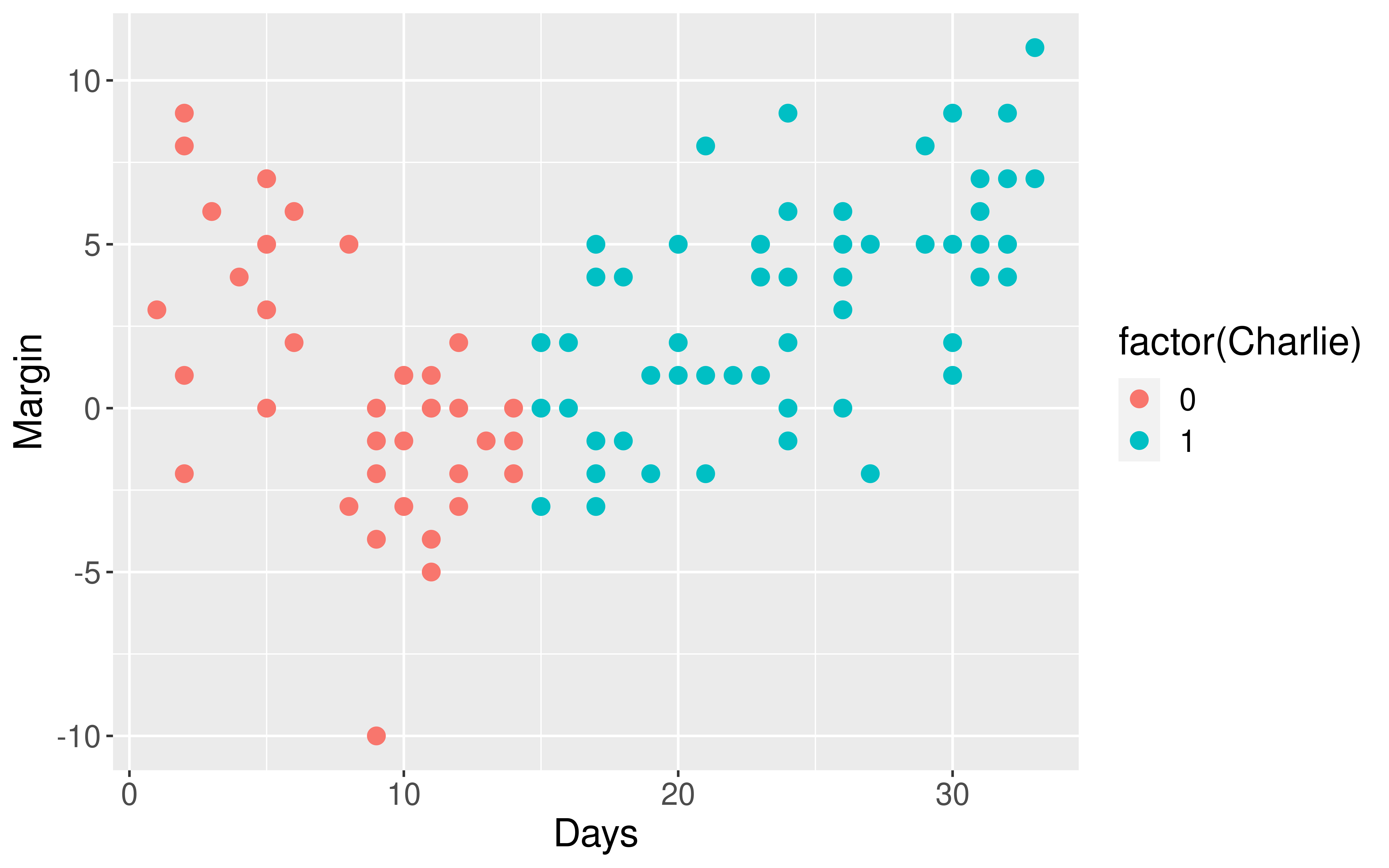
Is the assumption of equal slopes reasonable here?

Model Forms

Same Slopes Model:

Different Slopes Model:

• Line for \(x_2 = 1\):

• Line for \(x_2 = 0\):

Fitting the Linear Regression Model

modPoll <- lm(Margin ~ factor(Charlie)*Days, data = Pollster08)

get_regression_table(modPoll)

# A tibble: 4 × 7
  term                    estimate std_error statistic p_value lower_ci upper_ci
  <chr>                      <dbl>     <dbl>     <dbl>   <dbl>    <dbl>    <dbl>
1 intercept                  5.57      1.09       5.11       0    3.40     7.73 
2 factor(Charlie): 1       -10.1       1.92      -5.25       0  -13.9     -6.29 
3 Days                      -0.598     0.121     -4.96       0   -0.838   -0.359
4 factor(Charlie): 1:Days    0.921     0.136      6.75       0    0.65     1.19 

• Estimated regression line for \(x_2 = 1\):

• Estimated regression line for \(x_2 = 0\):

Adding the Regression Model to the Plot

ggplot(Pollster08, 
       aes(x = Days, 
           y = Margin, 
           color = factor(Charlie))) +
  geom_point(size = 3) +
  stat_smooth(method = lm, se = FALSE)

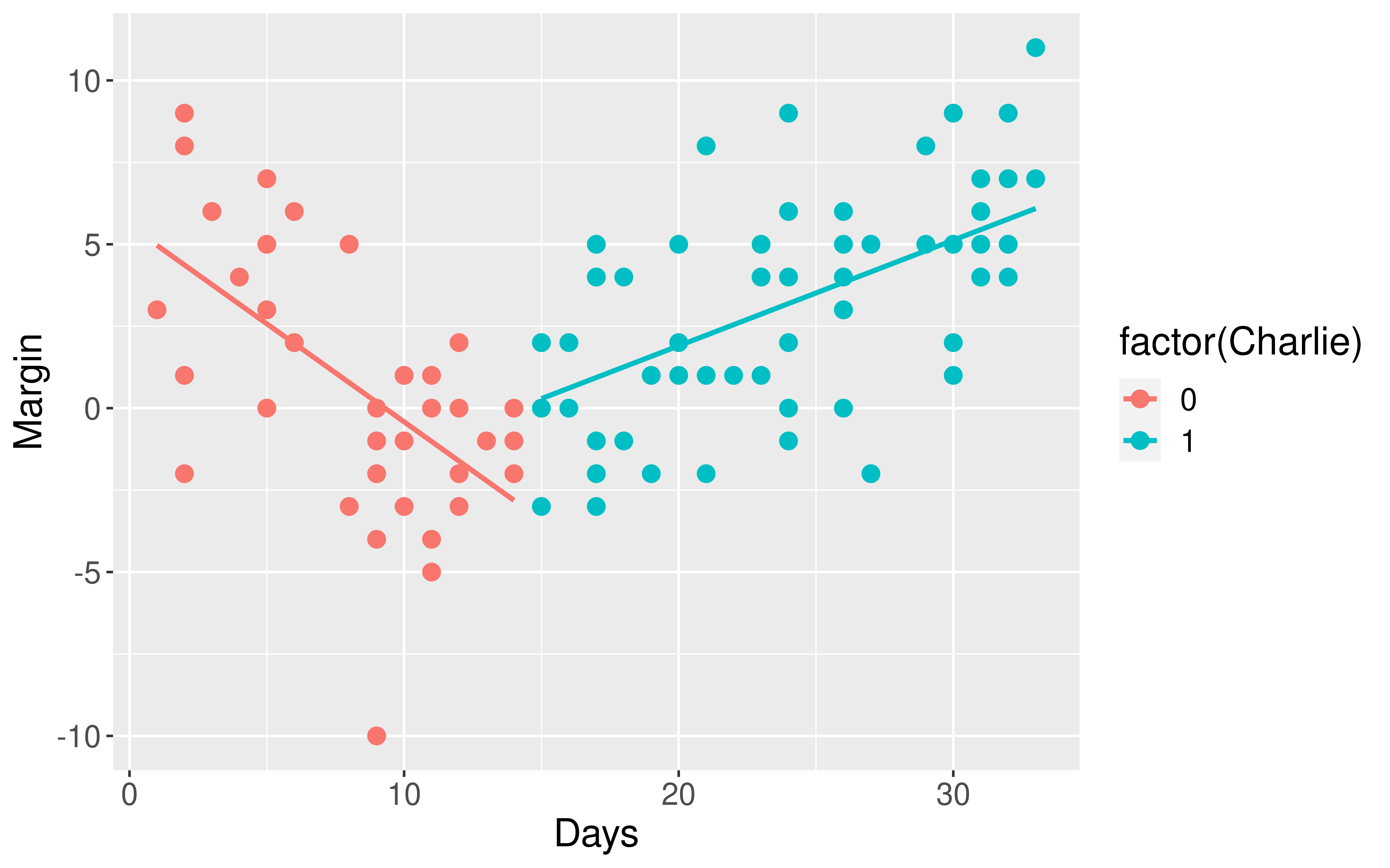
Is our modeling goal here predictive or descriptive?