Model Guidance

Kelly McConville

Stat 100
Week 8 | Fall 2023

Announcements

Oct 30th: Hex or Treat Day in Stat 100
- Wear a Halloween costume and get either a hex sticker or candy!!

Goals for Today

Finish up: Regression with polynomial explanatory variables
Modeling guidance

Sampling variability
Sampling distributions

Which Are You?

Data Visualizer

Data Wrangler

Model Builder

Linear Regression

Model Form:

\[ \begin{align} y &= \beta_o + \beta_1 x_1 + \beta_2 x_2 + \cdots + \beta_p x_p + \epsilon \end{align} \]

Linear regression is a flexible class of models that allow for:

Both quantitative and categorical explanatory variables.
Multiple explanatory variables.
Curved relationships between the response variable and the explanatory variable.
BUT the response variable is quantitative.

Example: Movies

Let’s model a movie’s critic rating using the audience rating and the movie’s genre.

library(tidyverse)
movies <- read_csv("https://www.lock5stat.com/datasets2e/HollywoodMovies.csv")

# Restrict our attention to dramas, horrors, and actions
movies2 <- movies %>%
  filter(Genre %in% c("Drama", "Horror", "Action")) %>%
  drop_na(Genre, AudienceScore, RottenTomatoes)
glimpse(movies2)

Rows: 313
Columns: 16
$ Movie            <chr> "Spider-Man 3", "Transformers", "Pirates of the Carib…
$ LeadStudio       <chr> "Sony", "Paramount", "Disney", "Warner Bros", "Warner…
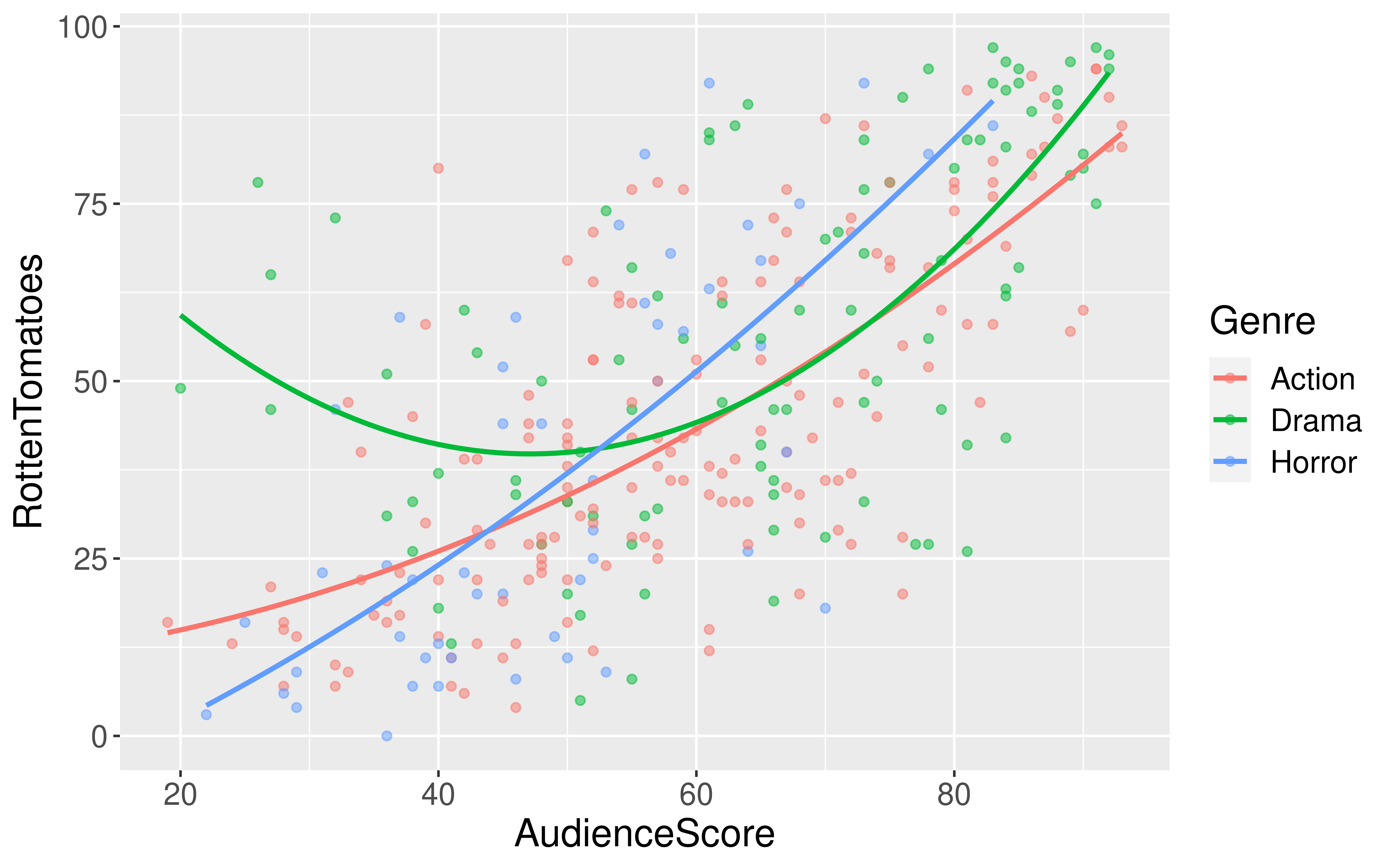
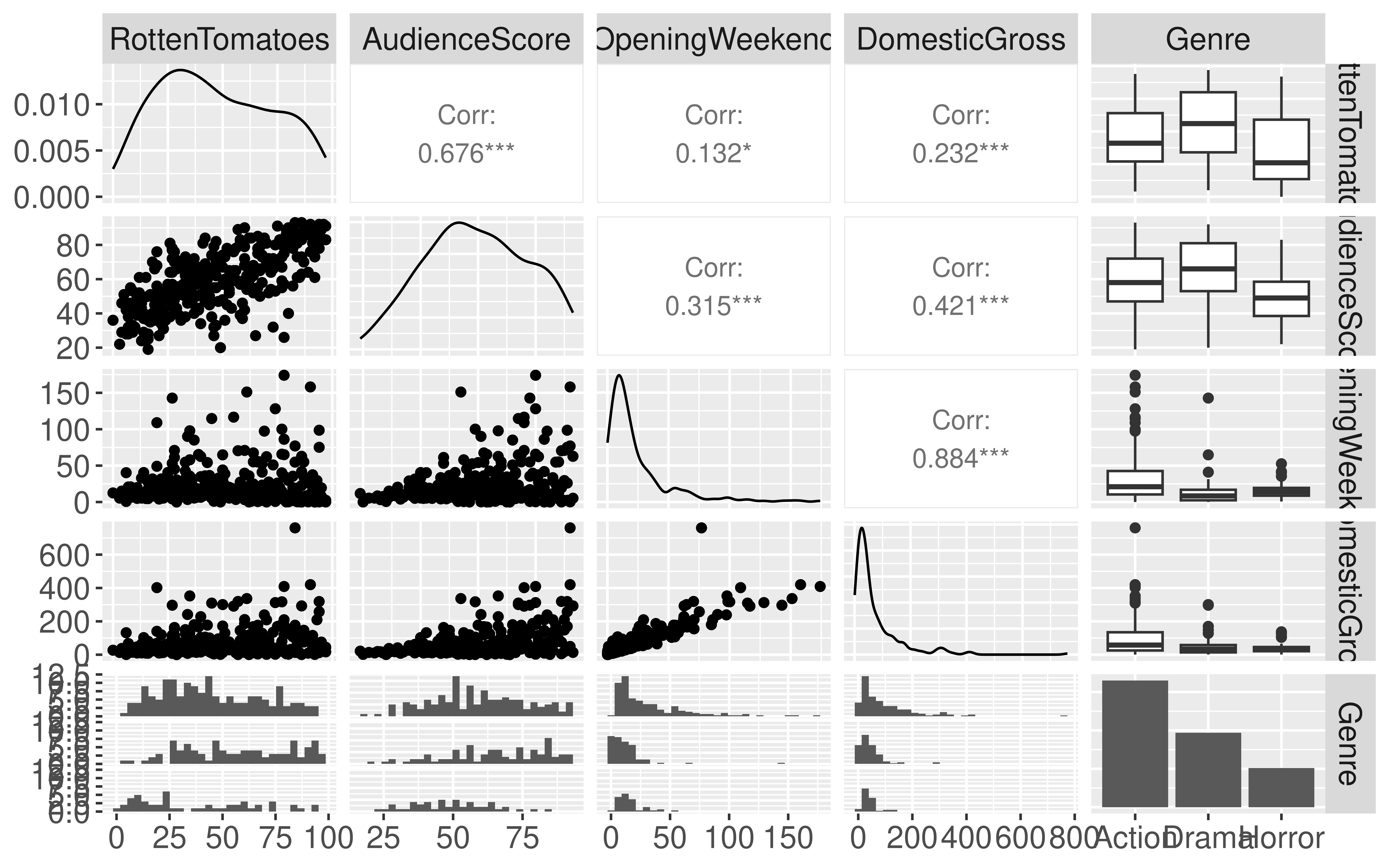
$ RottenTomatoes   <dbl> 61, 57, 45, 60, 20, 79, 35, 28, 41, 71, 95, 42, 18, 2…
$ AudienceScore    <dbl> 54, 89, 74, 90, 68, 86, 55, 56, 81, 52, 84, 55, 70, 6…
$ Story            <chr> "Metamorphosis", "Monster Force", "Rescue", "Sacrific…
$ Genre            <chr> "Action", "Action", "Action", "Action", "Action", "Ac…
$ TheatersOpenWeek <dbl> 4252, 4011, 4362, 3103, 3778, 3408, 3959, 3619, 2911,…
$ OpeningWeekend   <dbl> 151.1, 70.5, 114.7, 70.9, 49.1, 33.4, 58.0, 45.3, 19.…
$ BOAvgOpenWeekend <dbl> 35540, 17577, 26302, 22844, 12996, 9791, 14663, 12541…
$ DomesticGross    <dbl> 336.53, 319.25, 309.42, 210.61, 140.13, 134.53, 131.9…
$ ForeignGross     <dbl> 554.34, 390.46, 654.00, 245.45, 117.90, 249.00, 157.1…
$ WorldGross       <dbl> 890.87, 709.71, 963.42, 456.07, 258.02, 383.53, 289.0…
$ Budget           <dbl> 258.0, 150.0, 300.0, 65.0, 140.0, 110.0, 130.0, 110.0…
$ Profitability    <dbl> 345.30, 473.14, 321.14, 701.64, 184.30, 348.66, 222.3…
$ OpenProfit       <dbl> 58.57, 47.00, 38.23, 109.08, 35.07, 30.36, 44.62, 41.…
$ Year             <dbl> 2007, 2007, 2007, 2007, 2007, 2007, 2007, 2007, 2007,…

Coming Back to Our Exploratory Data Analysis

ggplot(data = movies2,
       mapping = aes(x = AudienceScore,
                     y = RottenTomatoes,
                     color = Genre)) +
  geom_point(alpha = 0.5) +
  stat_smooth(method = lm, se = FALSE, 
        formula = y ~ poly(x, degree = 2))

Fitting the Polynomial Model

mod2 <- lm(RottenTomatoes ~ poly(AudienceScore, degree = 2, raw = TRUE) + Genre, data = movies2)
library(moderndive)
get_regression_table(mod2, print = TRUE)

term	estimate	std_error	statistic	p_value	lower_ci	upper_ci
intercept	20.917	10.851	1.928	0.055	-0.434	42.267
poly(AudienceScore, degree = 2, raw = TRUE)1	-0.259	0.377	-0.687	0.492	-1.000	0.482
poly(AudienceScore, degree = 2, raw = TRUE)2	0.010	0.003	3.284	0.001	0.004	0.016
Genre: Drama	5.867	2.420	2.424	0.016	1.105	10.630
Genre: Horror	2.237	3.047	0.734	0.463	-3.758	8.233

Linear Regression & Curved Relationships

Form of the Model:

\[ \begin{align} y &= \beta_o + \beta_1 x_1 + \beta_2 x_2 + \cdots + \beta_p x_p + \epsilon \end{align} \]

But why is it called linear regression if the model also handles for curved relationship??

Model Building Guidance

What degree of polynomial should I include in my model?

Guiding Principle: Capture the general trend, not the noise.

\[ \begin{align} y &= f(x) + \epsilon \\ y &= \mbox{TREND} + \mbox{NOISE} \end{align} \]

Returning the 2008 Election Example:

Model Building Guidance

Shouldn’t we always include the interaction term?

Guiding Principle: Occam’s Razor for Modeling

“All other things being equal, simpler models are to be preferred over complex ones.” – ModernDive

Guiding Principle: Consider your modeling goals.

The equal slopes model allows us to control for the intensity of the light and then see the impact of being in the early or late timing groups on the number of flowers.

Later in the course will learn statistical procedures for determining whether or not a particular term should be included in the model.

What if I want to include more than 2 explanatory variables??

Model Building Guidance

We often have several potential explanatory variables. How do we determine which to include in the model and in what form?

Guiding Principle: Include explanatory variables that attempt to explain different aspects of the variation in the response variable.

library(GGally)
movies2 %>%
  select(RottenTomatoes, AudienceScore, OpeningWeekend, 
         DomesticGross, Genre) %>%
  ggpairs()

Model Building Guidance

We often have several potential explanatory variables. How do we determine which to include in the model and in what form?

Guiding Principle: Include explanatory variables that attempt to explain different aspects of the variation in the response variable.

mod_movies <- lm(RottenTomatoes ~ AudienceScore + DomesticGross + Genre, data = movies2)
get_regression_table(mod_movies, print = TRUE)

term	estimate	std_error	statistic	p_value	lower_ci	upper_ci
intercept	-12.472	4.083	-3.055	0.002	-20.506	-4.439
AudienceScore	0.975	0.072	13.590	0.000	0.834	1.117
DomesticGross	-0.006	0.015	-0.431	0.667	-0.035	0.023
Genre: Drama	6.117	2.644	2.314	0.021	0.916	11.319
Genre: Horror	2.058	3.141	0.655	0.513	-4.121	8.238

Model Building Guidance

We often have several potential explanatory variables. How do we determine which to include in the model and in what form?

Guiding Principle: Use your modeling motivation to determine how much you weigh interpretability versus prediction accuracy when choosing the model.

Model Building

We will come back to methods for model selection.
Key ideas:
- Determining the response variable and the potential explanatory variable(s)
- Writing out the model form and understanding the terms
- Building and visualizing linear regression models in R
- Comparing different potential models

Shift Gears: Statistical Inference

The ❤️ of statistical inference is quantifying uncertainty

library(tidyverse)
ce <- read_csv("data/fmli.csv")
summarize(ce, meanFINCBTAX = mean(FINCBTAX))

# A tibble: 1 × 1
  meanFINCBTAX
         <dbl>
1       62480.

The ❤️ of statistical inference is quantifying uncertainty

library(tidyverse)
ce <- read_csv("data/fmli.csv")
summarize(ce, meanFINCBTAX = mean(FINCBTAX))

# A tibble: 1 × 1
  meanFINCBTAX
         <dbl>
1       62480.

Now we need to distinguish between the population and the sample

Parameters:
- Based on the population
- Unknown then if don’t have data on the whole population
- EX: \(\beta_o\) and \(\beta_1\)
- EX: \(\mu\) = population mean

Statistics:
- Based on the sample data
- Known
- Usually estimate a population parameter
- EX: \(\hat{\beta}_o\) and \(\hat{\beta}_1\)
- EX: \(\bar{x}\) = sample mean

Quantifying Our Uncertainty

R has been giving us uncertainty estimates:

library(Stat2Data)
data("Pollster08")

ggplot(Pollster08, aes(x = Days,
                       y = Margin, 
                       color = factor(Charlie))) +
  geom_point() +
  stat_smooth(method = "lm", se = TRUE) +
  theme(legend.position = "bottom")

Quantifying Our Uncertainty

R has been giving us uncertainty estimates:

library(Stat2Data)
data("Pollster08")
modPoll <- lm(Margin ~ Days*factor(Charlie), data = Pollster08)
library(moderndive)
get_regression_table(modPoll)

# A tibble: 4 × 7
  term                  estimate std_error statistic p_value lower_ci upper_ci
  <chr>                    <dbl>     <dbl>     <dbl>   <dbl>    <dbl>    <dbl>
1 intercept                5.57      1.09       5.11       0    3.40     7.73 
2 Days                    -0.598     0.121     -4.96       0   -0.838   -0.359
3 factor(Charlie): 1     -10.1       1.92      -5.25       0  -13.9     -6.29 
4 Days:factor(Charlie)1    0.921     0.136      6.75       0    0.65     1.19