Grab 30 notecards! It is okay if they already have markings on them. And, please return the notecards to the same spot after class.
Confidence Intervals
Kelly McConville
Stat 100 Week 9 | Fall 2023
Announcements
Oct 30th Today: Hex or Treat Day in Stat 100
If you are wearing a Halloween costume, come to the front before or after class for your hex sticker or treat!
Goals for Today
Estimation
Bootstrap distributions
Bootstrapped confidence intervals
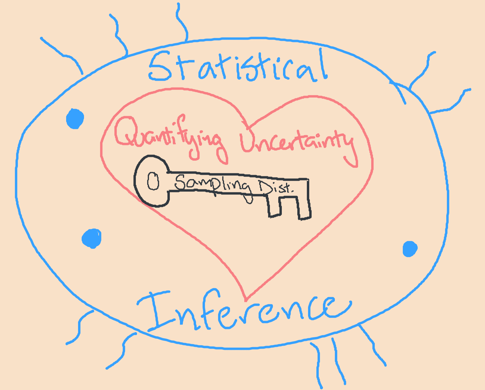
Question: How do sampling distributions help us quantify uncertainty?
Estimation
Goal: Estimate the value of a population parameter using data from the sample.
Sub-Goal: Quantify our uncertainty in using the sample to say something about the population.
Confidence Interval (CI): Interval of plausible values for a parameter
Form of a 95% Confidence Interval:
\[\begin{align*}
\mbox{statistic} &\pm \mbox{Margin of Error}\\
\mbox{statistic} &\pm 2\mbox{SE}
\end{align*}\]
Problem: To compute the SE, we need many samples from the population. We have 1 sample.
Solution: Approximate the sampling distribution using ONLY OUR ONE SAMPLE!
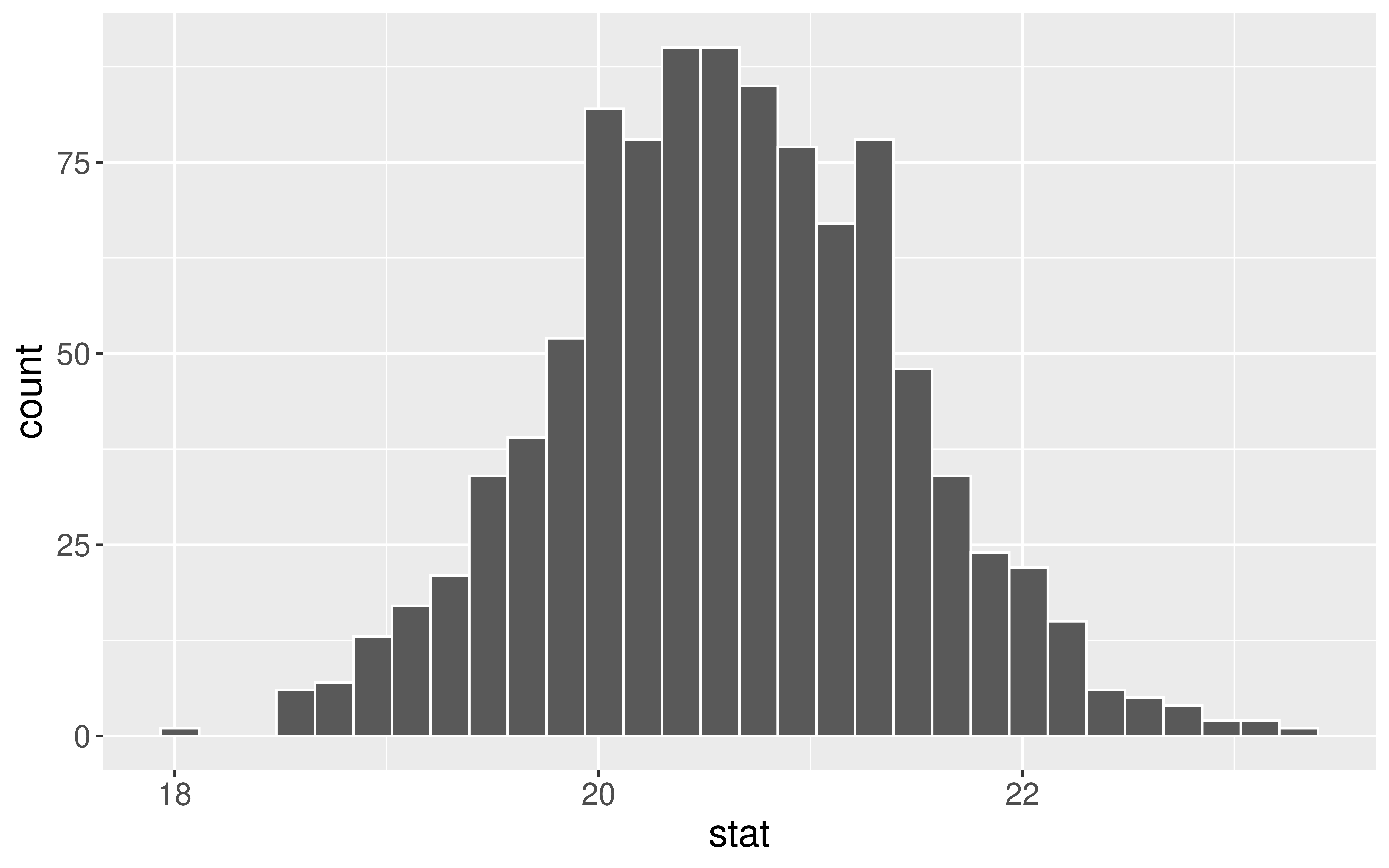
Bootstrap Distribution
How do we approximate the sampling distribution?
Bootstrap Distribution of a Sample Statistic:
Take a sample of size \(n\)with replacement from the sample. Called a bootstrap sample.
Compute the statistic on the bootstrap sample.
Repeat 1 and 2 many (1000+) times.
Let’s Practice Generating Bootstrap Samples!
Example: In a recent study, 23 rats showed compassion that surprised scientists. Twenty-three of the 30 rats in the study freed another trapped rat in their cage, even when chocolate served as a distraction and even when the rats would then have to share the chocolate with their freed companion. (Rats, it turns out, love chocolate.) Rats did not open the cage when it was empty or when there was a stuffed animal inside, only when a fellow rat was trapped. We wish to use the sample to estimate the proportion of rats that show empathy in this way.
Parameter:
Statistic:
Use your 30 cards to take a bootstrap sample. (Make sure to appropriately label them first!)
Compute the bootstrap statistic and put it on the class dotplot.
(Will use these data for one of the problems in the next p-set.)
Sampling Distribution Versus Bootstrap Distribution
Data needed:
Center:
Spread:
(Bootstrapped) Confidence Intervals
95% CI Form:
\[
\mbox{statistic} \pm 2\mbox{SE}
\]
We approximate \(\mbox{SE}\) with \(\widehat{\mbox{SE}}\) = the standard deviation of the bootstrapped statistics.
Caveats:
Assuming a random sample
Even with random samples, sometimes we get non-representative samples. Bootstrapping can’t fix that.
Assuming the bootstrap distribution is bell-shaped and symmetric
Bootstrapped Confidence Intervals
Two Methods
Assuming random sample and roughly bell-shaped and symmetric bootstrap distribution for both methods.
SE Method 95% CI:
\[
\mbox{statistic} \pm 2\widehat{\mbox{SE}}
\]
We approximate \(\mbox{SE}\) with \(\widehat{\mbox{SE}}\) = the standard deviation of the bootstrapped statistics.
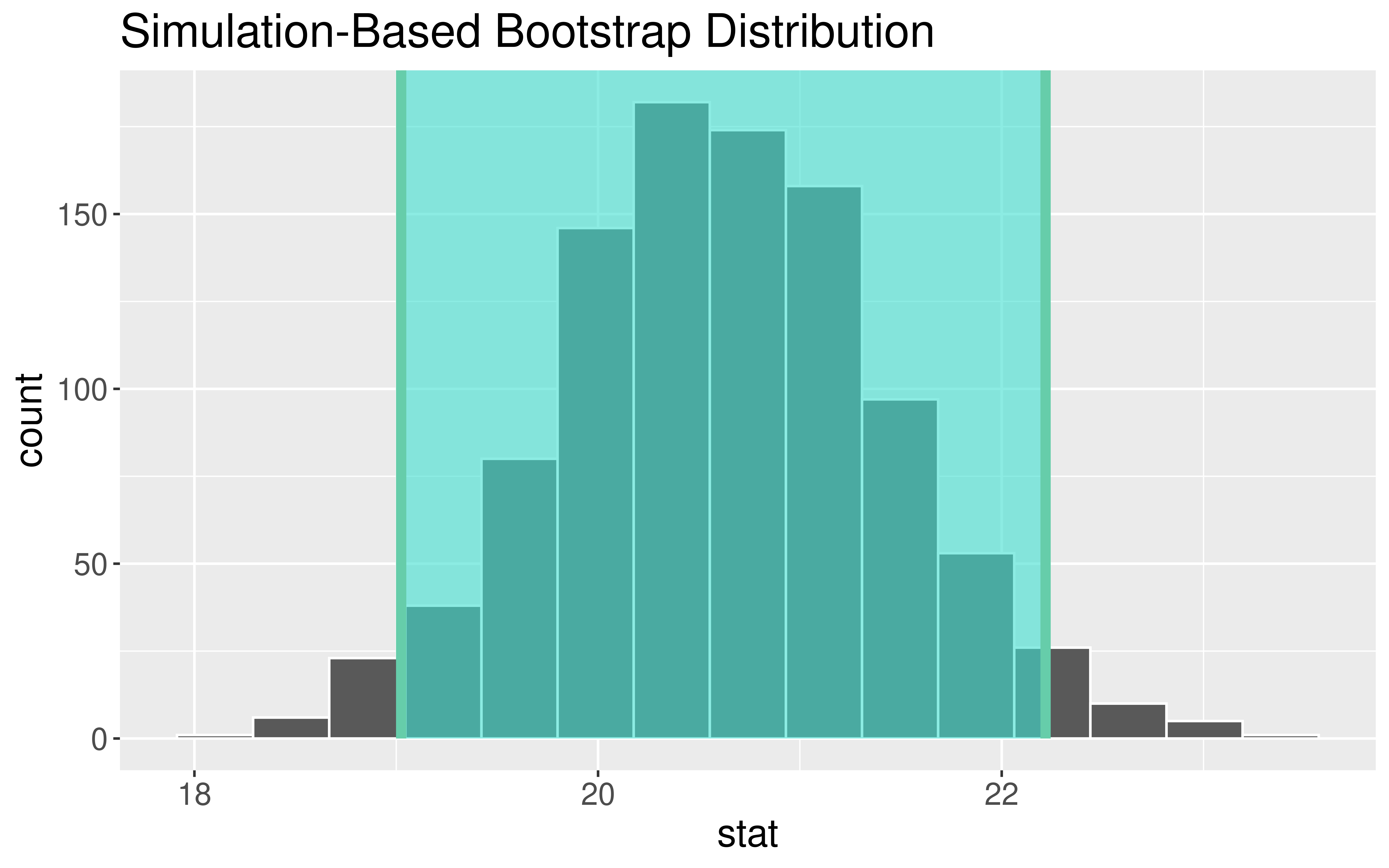
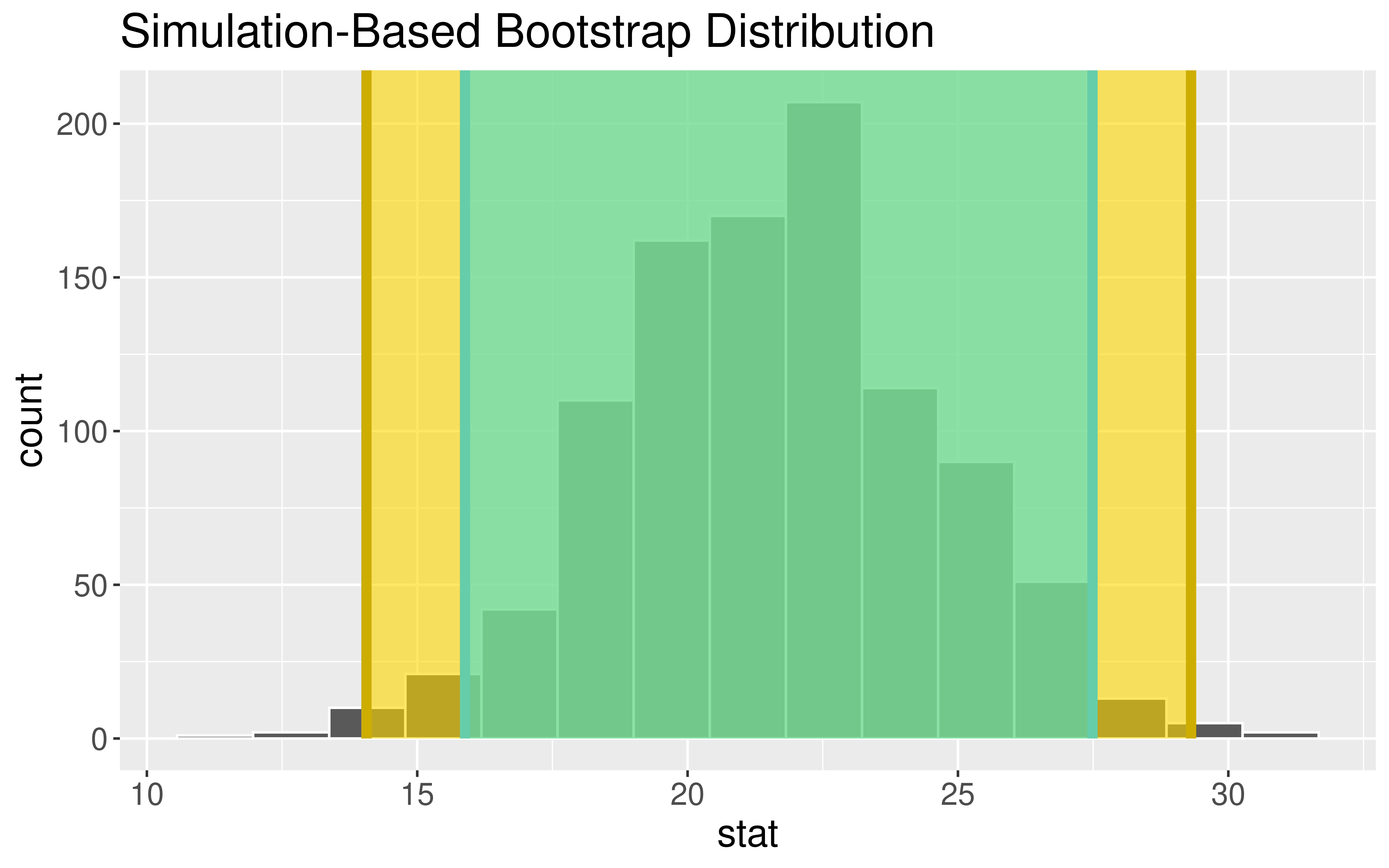
Percentile Method CI:
If I want a P% confidence interval, I find the bounds of the middle P% of the bootstrap distribution.
How can we construct bootstrap distributions and bootstrapped CIs in R?
Load Packages and Data
library(tidyverse)library(infer)
Let’s return to the movies dataset and estimate numerical quantities about Hollywood movies.
# Read in datamovies <-read_csv("https://www.lock5stat.com/datasets2e/HollywoodMovies.csv")
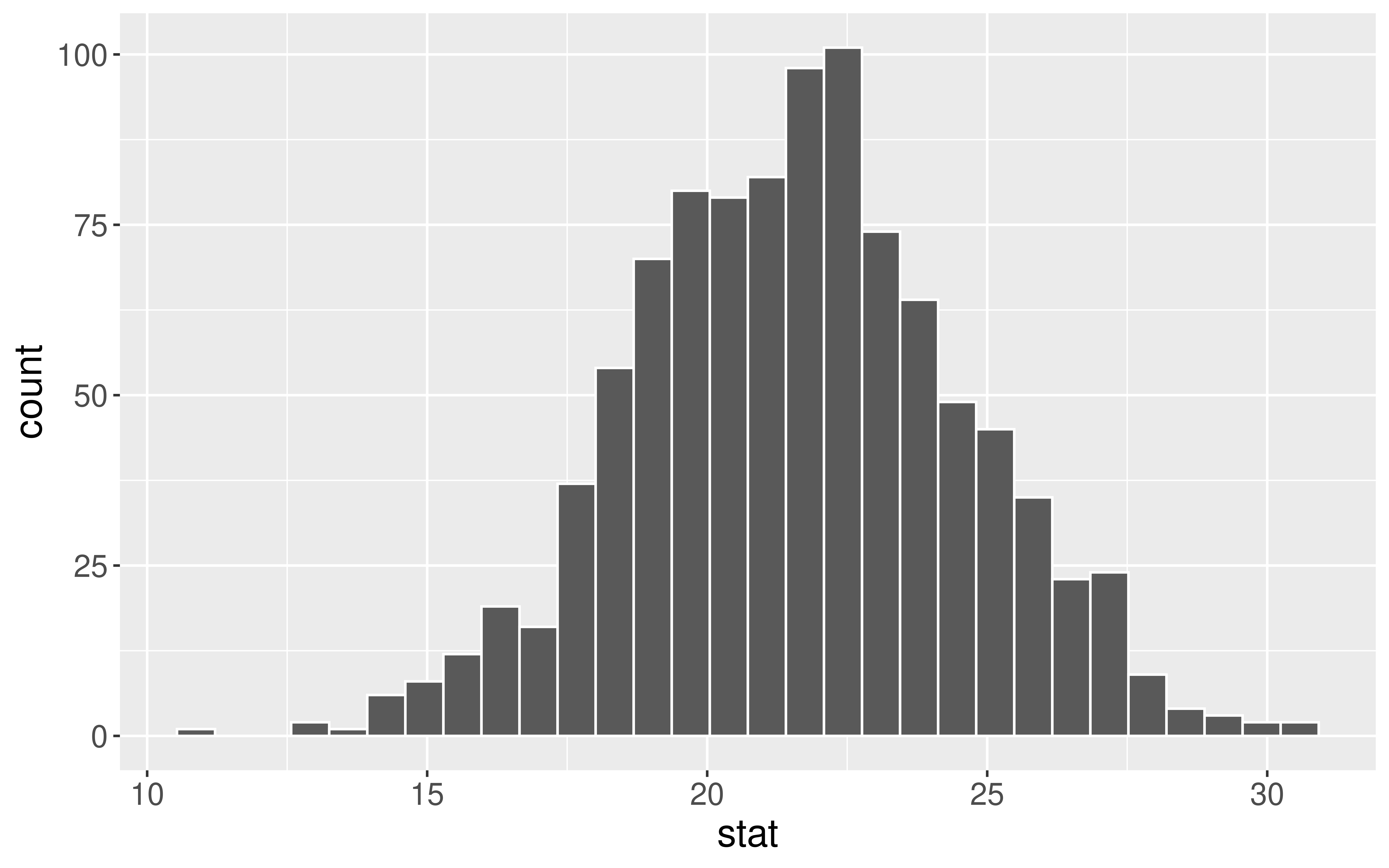
Estimation for a Single Mean
What is the average amount of money \((\mu)\) made in the opening weekend?
# Compute the summary statisticx_bar <- movies %>%drop_na(OpeningWeekend) %>%specify(response = OpeningWeekend) %>%calculate(stat ="mean")x_bar
Response: OpeningWeekend (numeric)
# A tibble: 1 × 1
   stat
  <dbl>
1  20.6
Why is our numerical quantity a mean and not a proportion or correlation here?
Estimation for a Single Mean
set.seed(999)# Construct bootstrap distributionbootstrap_dist <- movies %>%drop_na(OpeningWeekend) %>%specify(response = OpeningWeekend) %>%generate(reps =1000, type ="bootstrap") %>%calculate(stat ="mean")# Look at bootstrap distributionggplot(data = bootstrap_dist, mapping =aes(x = stat)) +geom_histogram(color ="white")
Interpretation: The point estimate is $ 20.6M. I am 95% confidence that the average amount of money made by all Hollywood movies is between $ 19M and $ 22.2M.
Inline R code: The point estimate is $ 20.6M. I am 95% confidence that the average amount of money made by all Hollywood movies is between $ 19.0243721 M and $ 22.2 M.
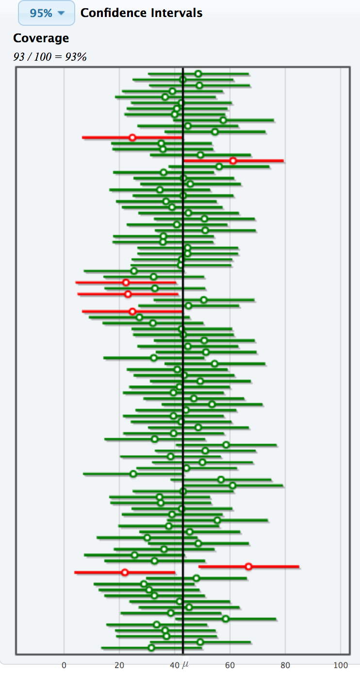
Confidence level = success rate of the method under repeated sampling
How do I know if my ONE CI successfully contains the true value of the parameter?
As we increase the confidence level, what happens to the width of the interval?
As we increase the sample size, what happens to the width of the interval?
As we increase the number of bootstrap samples we take, what happens to the width of the interval?
Interpreting Confidence Intervals
Example: Estimating average household income before taxes in the US
SE Method Formula:
\[
\mbox{statistic} \pm{\mbox{ME}}
\]
# A tibble: 1 × 3
     ME  lower  upper
  <dbl>  <dbl>  <dbl>
1 1963. 60517. 64443.
“The margin of [sampling] error can be described as the ‘penalty’ in precision for not talking to everyone in a given population. It describes the range that an answer likely falls between if the survey had reached everyone in a population, instead of just a sample of that population.” – Courtney Kennedy, Director of Survey Research at Pew Research Center
CI = interval of plausible values for the parameter
Safe interpretation: I am P% confident that {insert what the parameter represents in context} is between {insert lower bound} and {insert upper bound}.
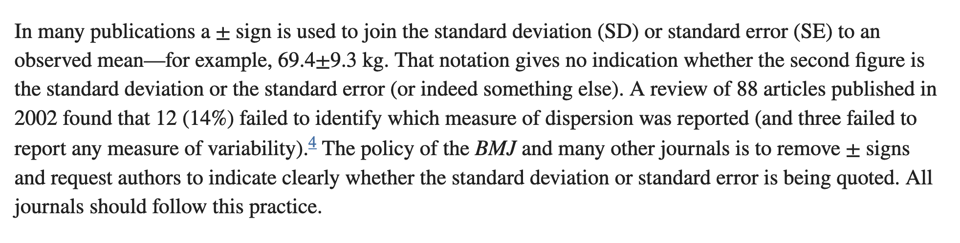
Caution: Confidence intervals in the wild
Statement in an article for The BMJ (British Medical Journal):
🤔 The second half of Stat 100 is more conceptually difficult. 🤔
So keep coming to lecture, to section, to wrap-up sessions, and to office hours to get your questions answered!
Reminders:
Oct 30th Today: Hex or Treat Day in Stat 100
If you are wearing a Halloween costume, come to the front before or after class for your hex sticker or treat!