🎉 We are now accepting Course Assistant/Teaching Fellow applications for Stat 100 for next semester. To apply, fill out this application by Nov 15th.
No wrap-up session on Friday due to the university holiday.
You are all invited to the Info Session on Data Science Internships: Mon at 4pm in SC 316!
Goals for Today
Coding goals (Stat 100 & beyond)
Advice on the next stats/coding class
Decisions in a hypothesis test
Types of errors
The power of a hypothesis test
Now that you are at least 25% of the way to a stats secondary, what other classes should you consider?
That Next Stats Class
But first… Common Question: How should I describe my post-Stat 100 coding abilities?
Potential Answer: You have learned how to write code to analyze data. This includes visualization (ggplot2), data wrangling (dplyr), data importation (readr), modeling, inference (infer) and communication (with Quarto).
Follow-up Question: So what coding is there left to learn?
Answer: Learning how to program. This includes topics such as control flow, iteration, creating functions, and vectorization.
That Next Coding Class
Stat 108: Introduction to Statistical Computing with R
CompSci 32: Computational Thinking and Problem Solving
CompSci 50: Introduction to Computer Science
AP 10: Computing with Python for Scientists and Engineers
That Next Modeling Course
Stat 109A: Data Science I & Stat 109B: Data Science II
Stat 139: Linear Models
Many of the upper-level stats courses are modeling courses (but they do have pre-reqs).
That Next Theory/Methods Course
Stat 110: Introduction to Probability
Stat 111: Introduction to Statistical Inference
That Next Visualization Course
Stat 108: Introduction to Statistical Computing with R
CompSci 171: Visualization
Stat 106: Data Science for Sports Analytics
Not on the books yet but should be coming next academic year.
Another Hypothesis Testing Example
Penguins Example
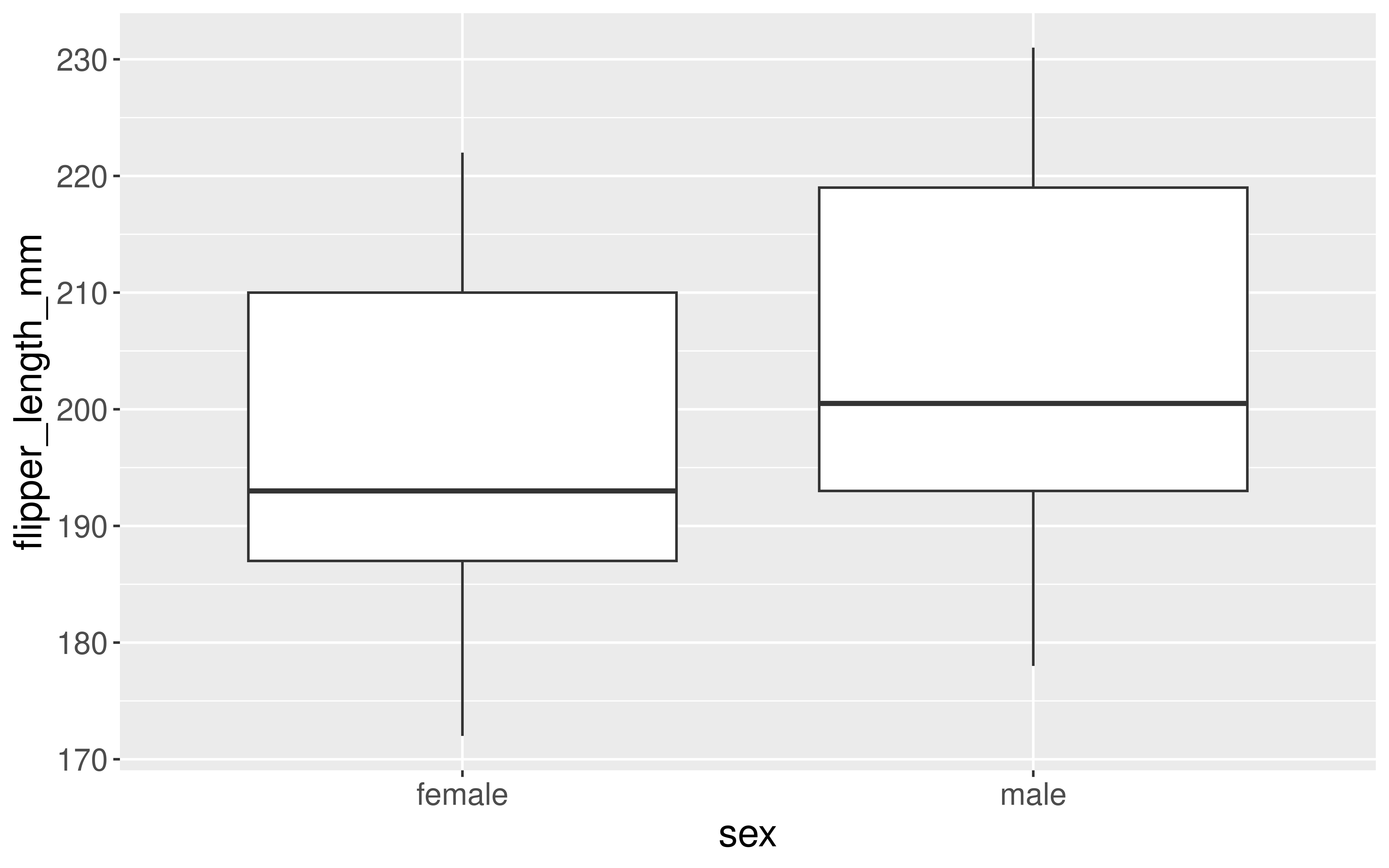
Let’s return to the penguins data and ask if flipper length varies, on average, by the sex of the penguin.
Research Question: Does flipper length differ by sex?
Interpretation of\(p\)-value: If the mean flipper length does not differ by sex in the population, the probability of observing a difference in the sample means of at least 7.142316 mm (in magnitude) is equal to 0.
Conclusion: These data represent evidence that flipper length does vary by sex.
Hypothesis Testing: Decisions, Decisions
Once you get to the end of a hypothesis test you make one of two decisions:
P-value is small.
I have evidence for \(H_a\). Reject \(H_o\).
P-value is not small.
I don’t have evidence for \(H_a\). Fail to reject \(H_o\).
Sometimes we make the correct decision. Sometimes we make a mistake.
Hypothesis Testing: Decisions, Decisions
Let’s create a table of potential outcomes.
\(\alpha\) = prob of Type I error under repeated sampling = prob reject \(H_o\) when it is true
\(\beta\) = prob of Type II error under repeated sampling = prob fail to reject \(H_o\) when \(H_a\) is true.
Hypothesis Testing: Decisions, Decisions
Typically set \(\alpha\) level beforehand.
Use \(\alpha\) to determine “small” for a p-value.
P-value issmall\(< \alpha\).
I have evidence for \(H_a\). Reject \(H_o\).
P-value isnotsmall\(\geq \alpha\).
I don’t have evidence for \(H_a\). Fail to reject \(H_o\).
Hypothesis Testing: Decisions, Decisions
Question: How do I select \(\alpha\)?
Will depend on the convention in your field.
Want a small \(\alpha\) and a small \(\beta\). But they are related.
The smaller\(\alpha\) is the larger \(\beta\) will be.
Choose a lower \(\alpha\) (e.g., 0.01, 0.001) when the Type I error is worse and a higher \(\alpha\) (e.g., 0.1) when the Type II error is worse.
Can’t easily compute \(\beta\). Why?
One more important term:
Power = probability reject \(H_o\) when the alternative is true.
Example
Suppose we have a baseball player who has been a 0.250 career hitter who suddenly improves to be a 0.333 hitter. He wants a raise but needs to convince his manager that he has genuinely improved. The manager offers to examine his performance in 20 at-bats.
Ho:
Ha:
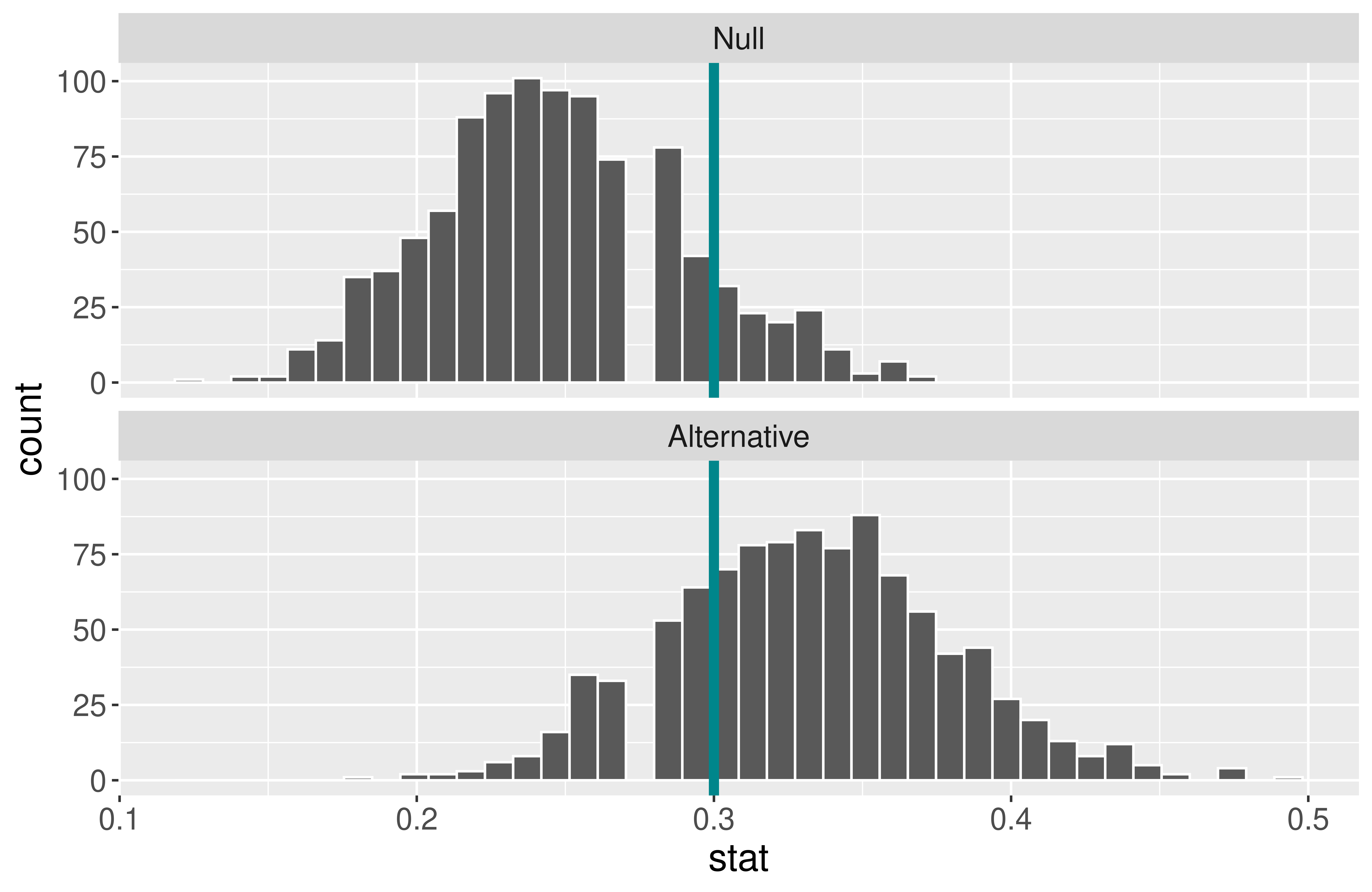
When \(\alpha\) is set to \(0.05\), he needs to hit 9 or more to get a small enough p-value to reject \(H_o\).
When \(\alpha\) is set to \(0.05\), the power of this test is 0.204.
Why is the power so low?
What aspects of the test could the baseball player change to increase the power of the test?
Example
Suppose we have a baseball player who has been a 0.250 career hitter who suddenly improves to be a 0.333 hitter. He wants a raise but needs to convince his manager that he has genuinely improved. The manager offers to examine his performance in 20 100 at-bats.
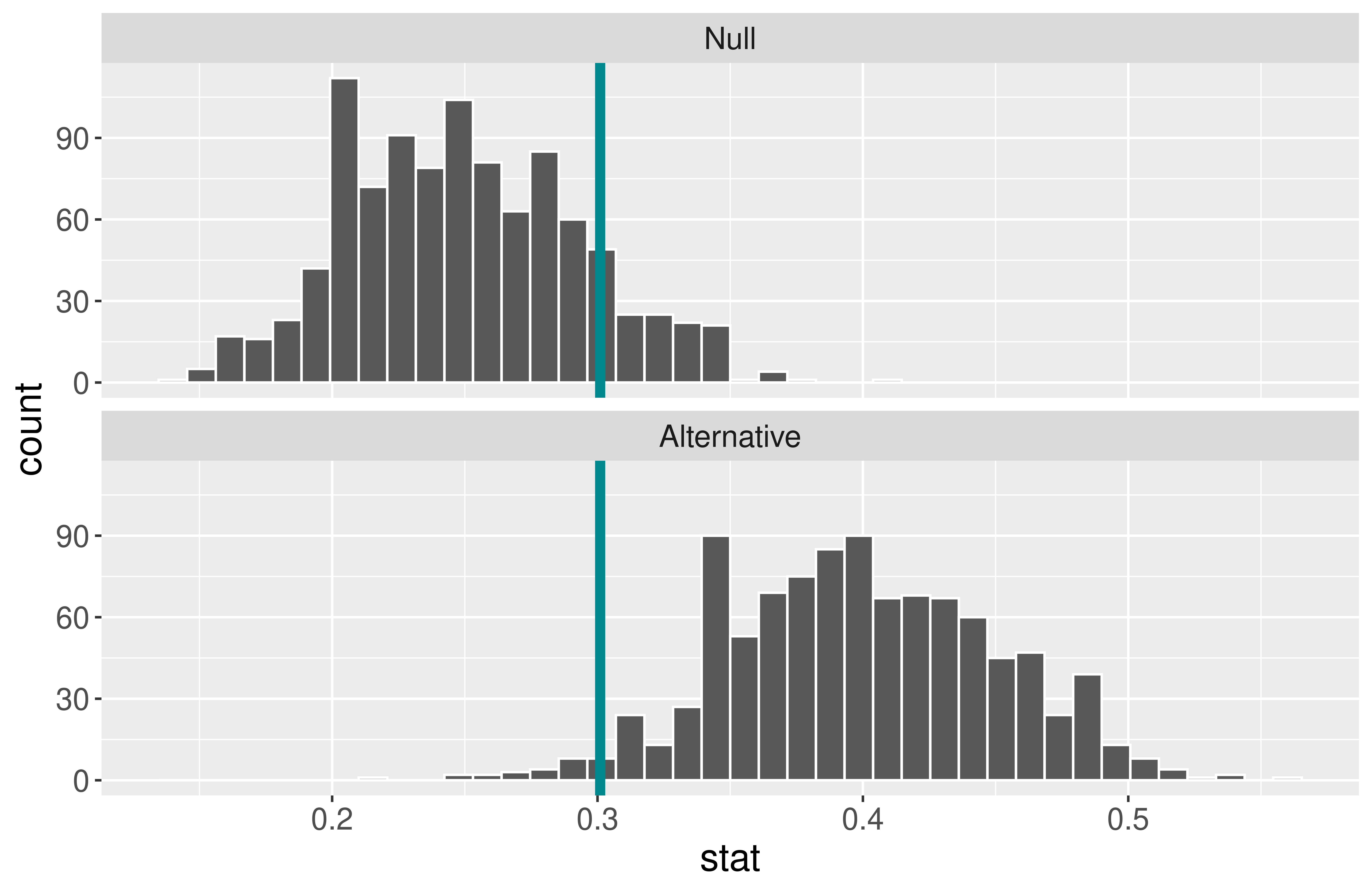
What will happen to the power of the test if we increase the sample size?
Increasing the sample size increases the power.
When \(\alpha\) is set to \(0.05\) and the sample size is now 100, the power of this test is 0.57.
Example
Suppose we have a baseball player who has been a 0.250 career hitter who suddenly improves to be a 0.333 hitter. He wants a raise but needs to convince his manager that he has genuinely improved. The manager offers to examine his performance in 20 100 at-bats.
What will happen to the power of the test if we increase\(\alpha\) to 0.1?
Increasing \(\alpha\) increases the power.
Decreases \(\beta\).
When \(\alpha\) is set to \(0.1\) and the sample size is 100, the power of this test is 0.71.
Example
Suppose we have a baseball player who has been a 0.250 career hitter who suddenly improves to be a 0.333 0.400 hitter. He wants a raise but needs to convince his manager that he has genuinely improved. The manager offers to examine his performance in 20 100 at-bats.
What will happen to the power of the test if he is an even better player?
Effect size: Difference between true value of the parameter and null value.
Often standardized.
Increasing the effect size increases the power.
When \(\alpha\) is set to \(0.1\), the sample size is 100, and the true probability of hitting the ball is 0.4, the power of this test is 0.97.
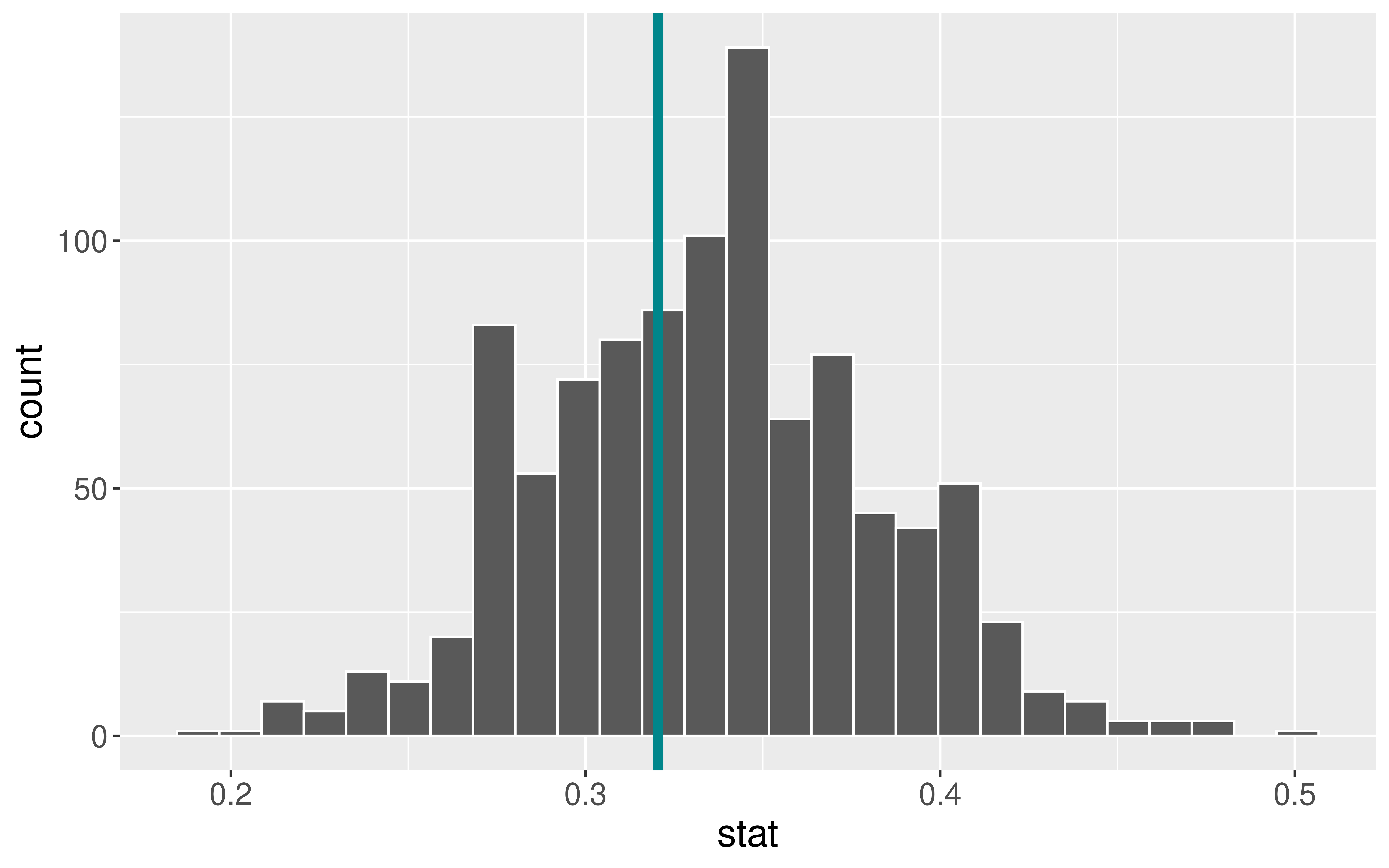
Computing Power
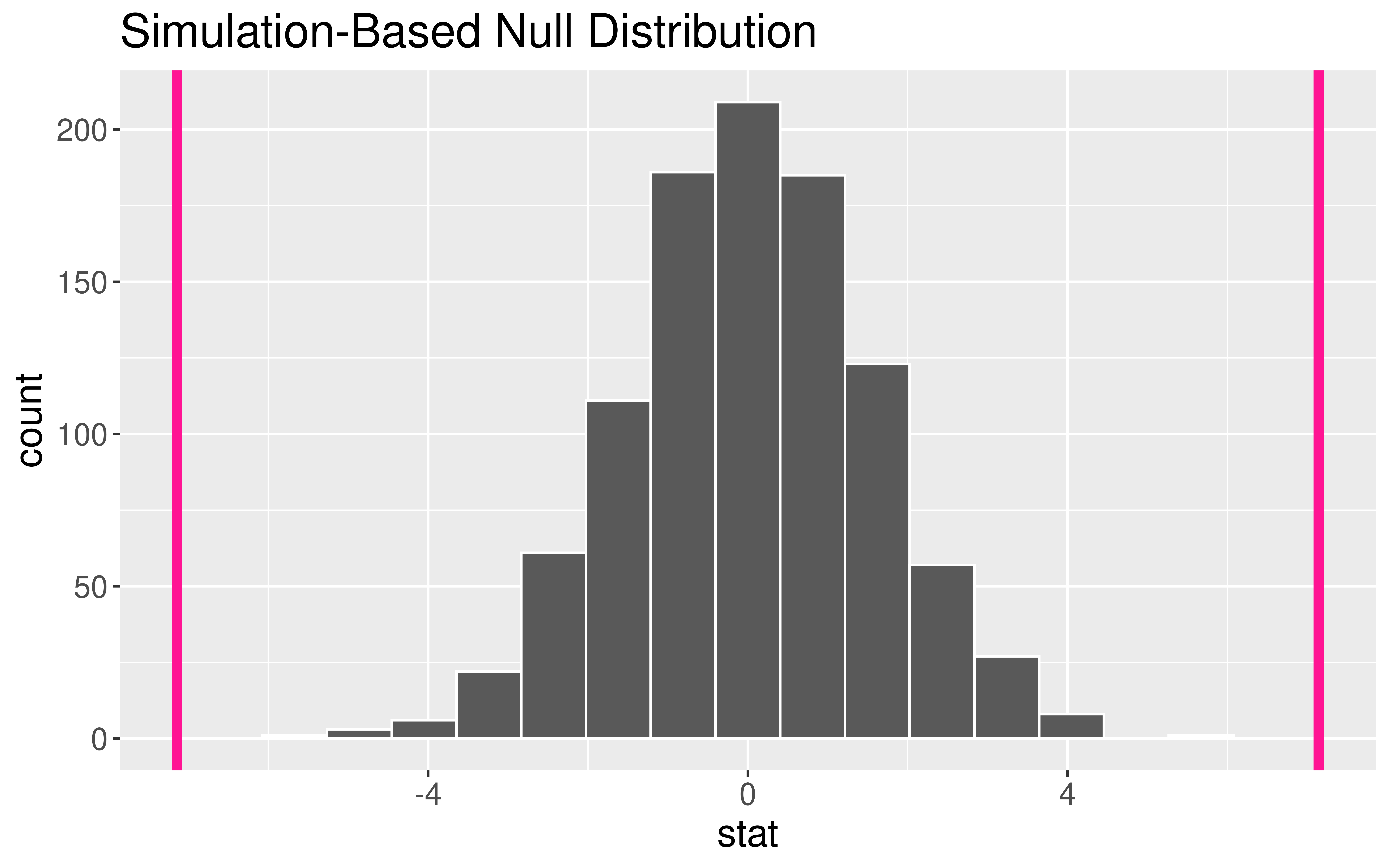
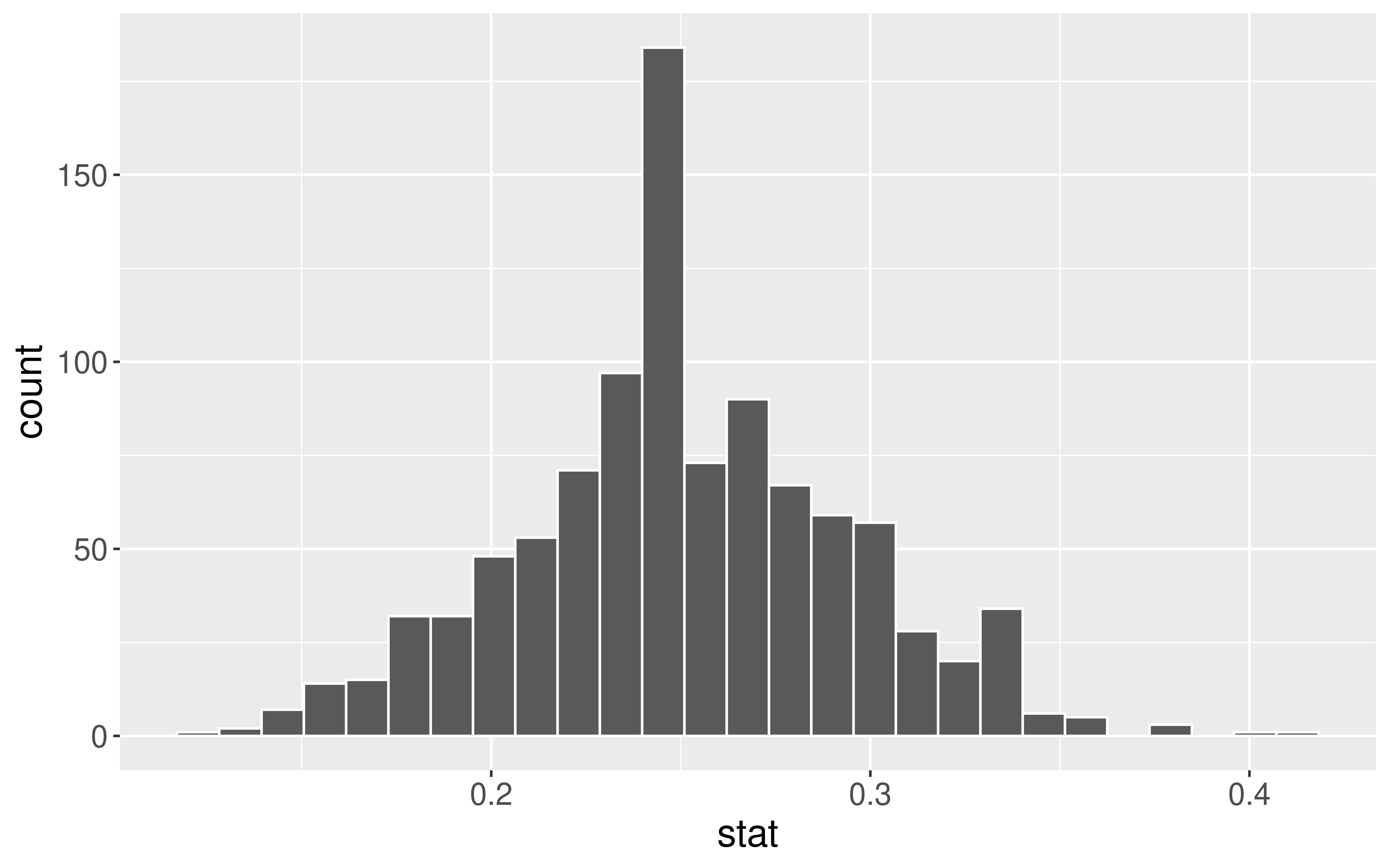
Generate a null distribution:
# Create a dummy dataset with the correct sample sizedat <-data.frame(at_bats =c(rep("hit", 80), rep("miss", 20)))null <- dat %>%specify(response = at_bats, success ="hit") %>%hypothesize(null ="point", p =0.25) %>%generate(reps =1000, type ="draw") %>%calculate(stat ="prop")ggplot(data = null, mapping =aes(x = stat)) +geom_histogram(bins =27, color ="white")
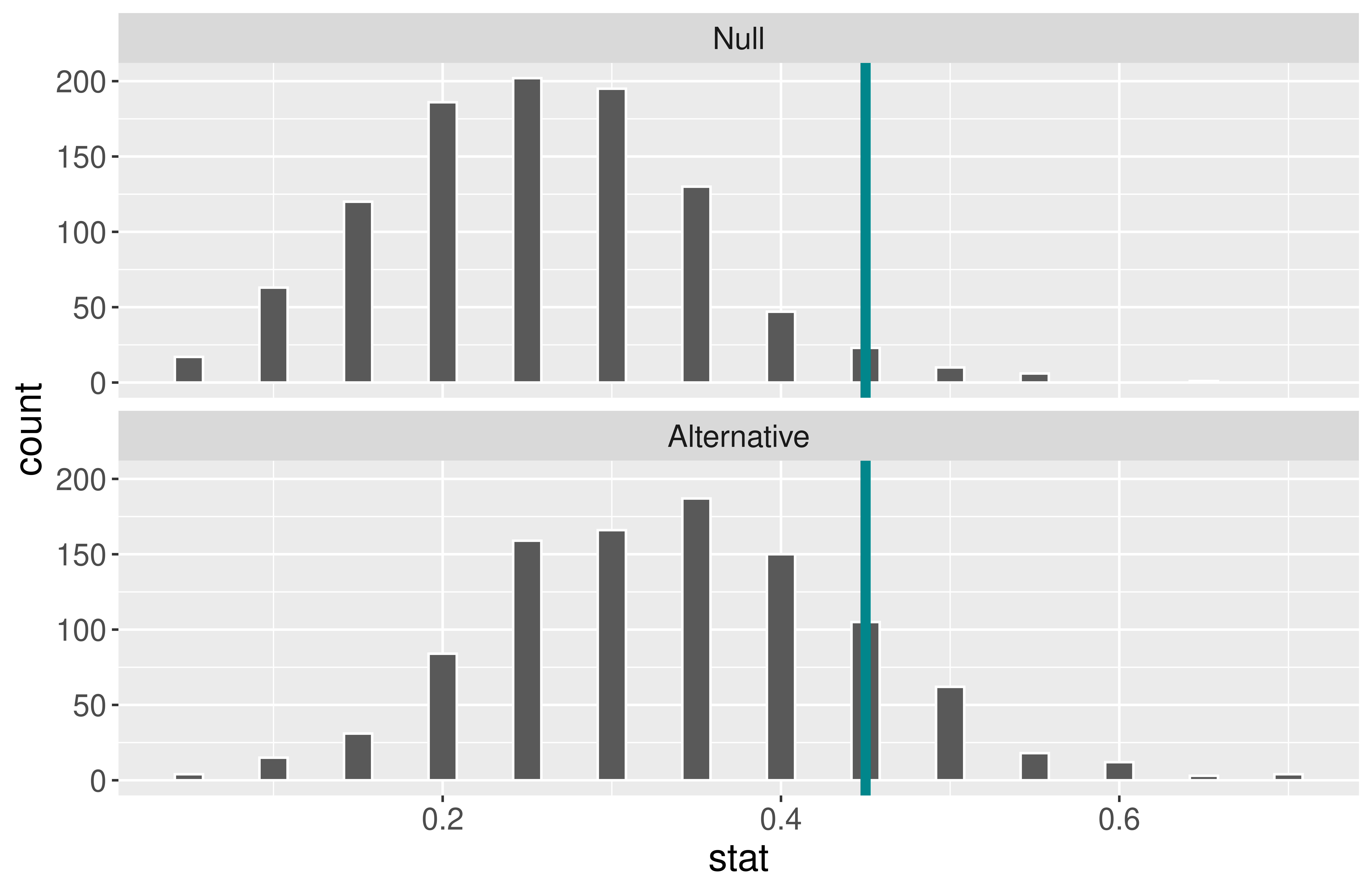
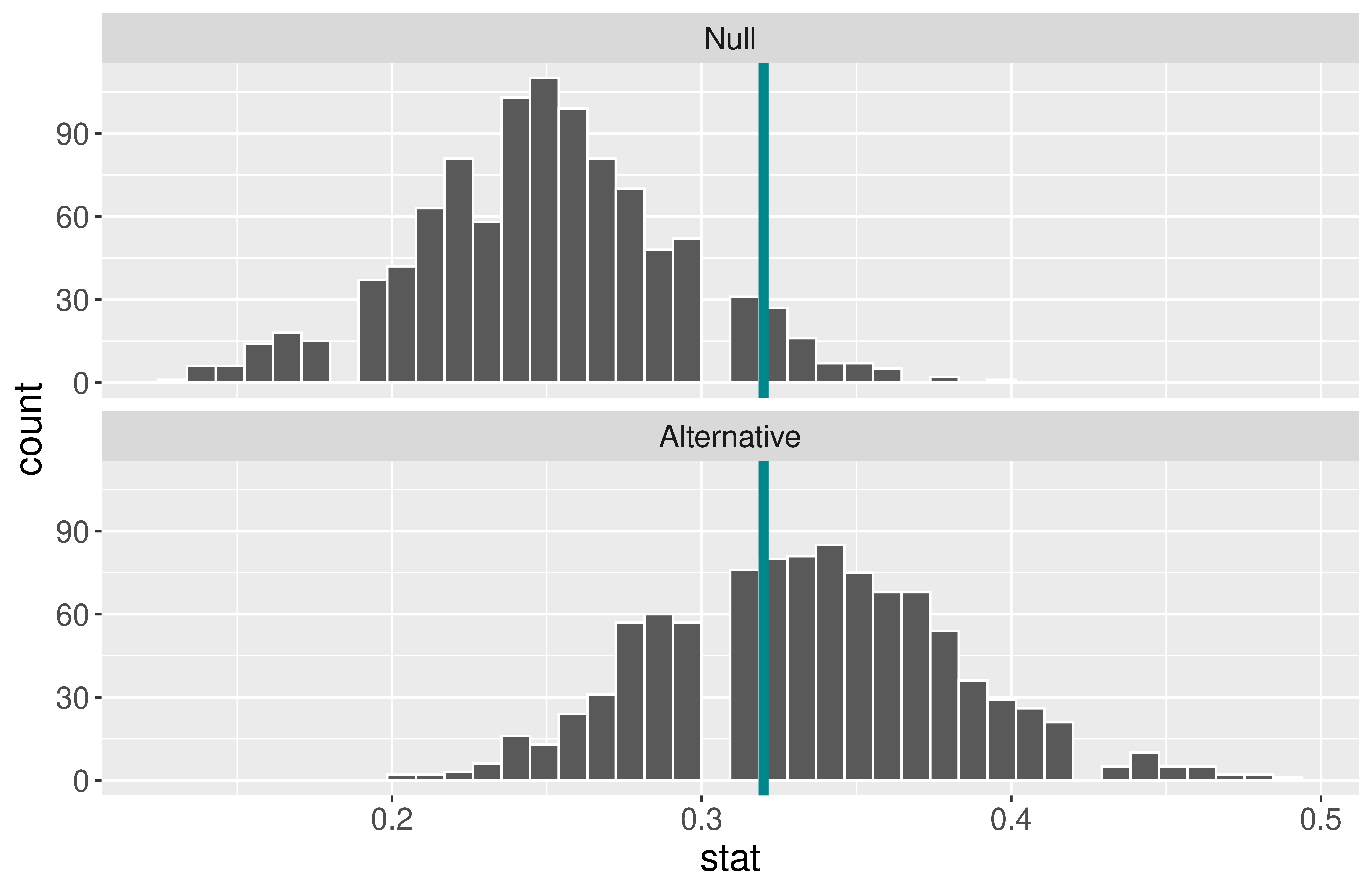
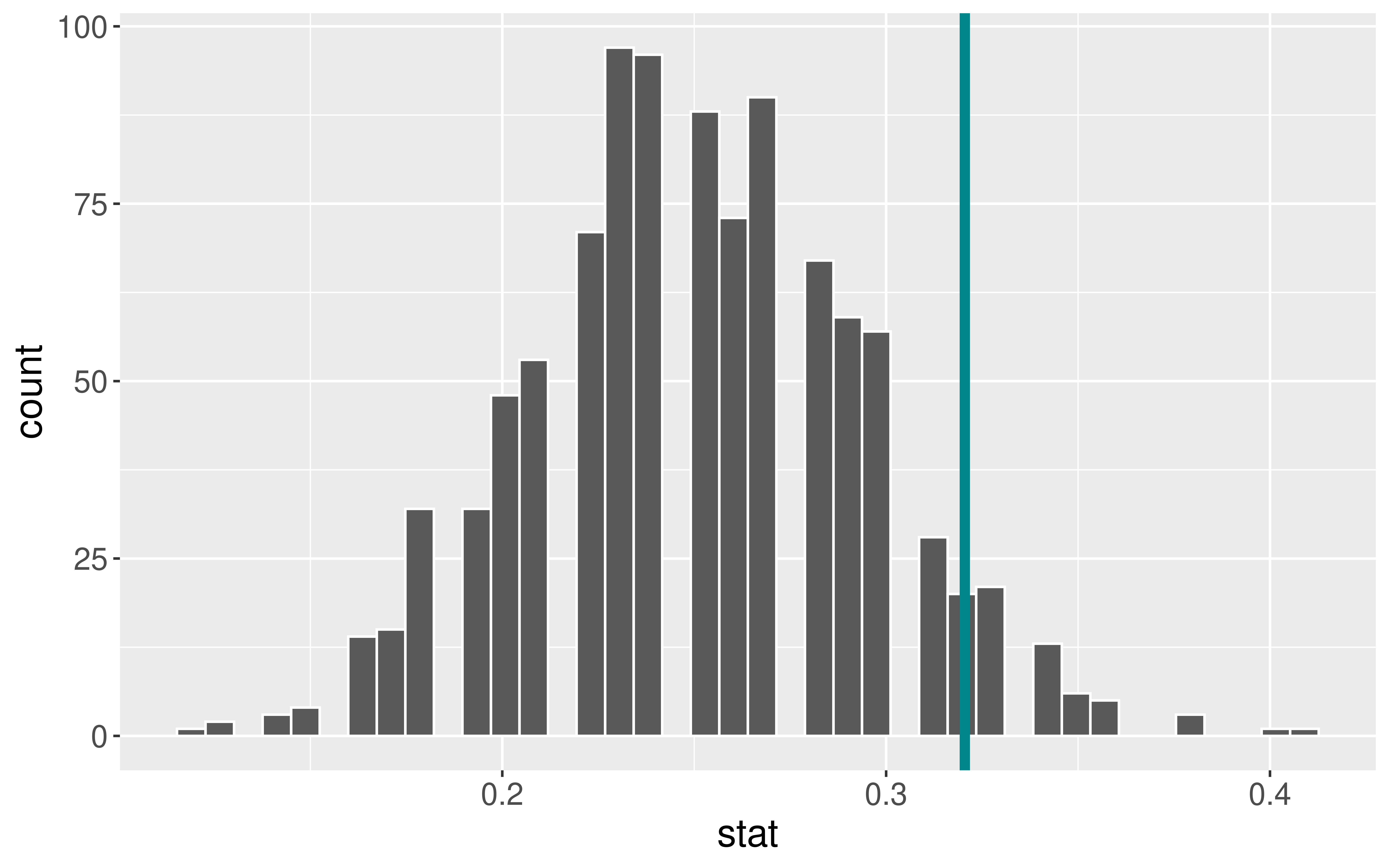
Computing Power
Determine the “critical value(s)” where \(\alpha = 0.05\)