Probability Concepts
Kelly McConville
Stat 100
Week 11 | Fall 2023
Announcements
- Only Thursday wrap-ups this week!
- No sections or wrap-ups during Thanksgiving Week.
- OH schedule for Thanksgiving Week:
Goals for Today
Conditional Probabilities
“Conditioning is the soul of statistics.” — Joe Blitzstein, Stat 110 Prof
Question: What do we mean by “conditioning”?
- Most polar bears are twins. Therefore, if you’re a twin, you’re probably a polar bear.
- P(twin given polar bear) \(\neq\) P(polar bear given twin)
- The p-value is a conditional probability.
- P-value = P(data given \(H_o\)) ( \(\neq\) P( \(H_o\) given data))
Conditional Probabilities
Other favorite examples:
- P(have COVID given wear mask) \(\neq\) P(wear mask given have COVID)
- In a CDC study, P(wear mask given have COVID) = 0.71 while P(have COVID given wear mask) is much lower.
- P(it is raining given there are clouds directly overhead) \(\neq\) Pr(there are clouds directly overhead given it is raining)
Notation: P(A given B) = P(A | B)
Example
Testing for COVID-19 was an important part of the Keep Harvard Healthy Program. There are a variety of COVID-19 tests out there but for this problem let’s assume the following:
- The test gives a false negative result 13% of the time where a false negative case is a person with COVID-19 but the test says they don’t have it.
- The test gives a false positive result 5% of the time where a false positive case is a person who doesn’t have COVID-19 but the test says they do.
Let’s assume the true prevalence is 1%. During the 2021-2022 school year, each week they tested about 30,000 Harvard affiliates. Use the assumed percentages to fill in the following table of potential outcomes:
| Actually have COVID-19 |
|
|
|
| Actually don’t have COVID-19 |
|
|
|
| Total |
|
|
30,000 |
P(test - | have COVID) =
P(have COVID | test -) =
P(test + | don’t have COVID) =
P(don’t have COVID | test +) =
Example
The false negative rate of COVID-19 tests have varied wildly. One paper estimated it could be as high as 54%.
Recreate the table with this new false negative rate.
| Actually have COVID-19 |
|
|
|
| Actually don’t have COVID-19 |
|
|
|
| Total |
|
|
30,000 |
P(test - | have COVID) =
P(have COVID | test -) =
P(test + | don’t have COVID) =
P(don’t have COVID | test +) =
Random Variables
For a discrete random variable, care about its:
- Spread – Variance & Standard Deviation:
\[
\sigma^2 = \sum (x - \mu)^2 p(x)
\]
\[
\sigma = \sqrt{ \sum (x - \mu)^2 p(x)}
\]
Random Variables
If a random variable, \(X\), is a continuous RV, then it can take on any value in an interval.
\[
p(x) \color{orange}{\approx} P(X = x)
\]
but if \(p(4) > p(2)\) that still means that X is more likely to take on values around 4 than values around 2.
Random Variables: Continuous
Change \(\sum\) to \(\int\):
\(\int p(x) dx = 1\).
Center – Mean/Expected value:
\[
\mu = \int x p(x) dx
\]
Random Variables: Continuous
Change \(\sum\) to \(\int\):
Spread – Standard deviation:
\[
\sigma = \sqrt{ \int (x - \mu)^2 p(x) dx}
\]
Why do we care about random variables?
We will recast our sample statistics as random variables.
Use the distribution of the random variable to approximate the sampling distribution of our sample statistic!
Specific Named Random Variables
Specific Named Random Variables
There is a vast array of random variables out there.
But there are a few particular ones that we will find useful.
- Because these ones are used often, they have been given names.
Will identify these named RVs using the following format:
\[
X \sim \mbox{Name(values of key parameters)}
\]
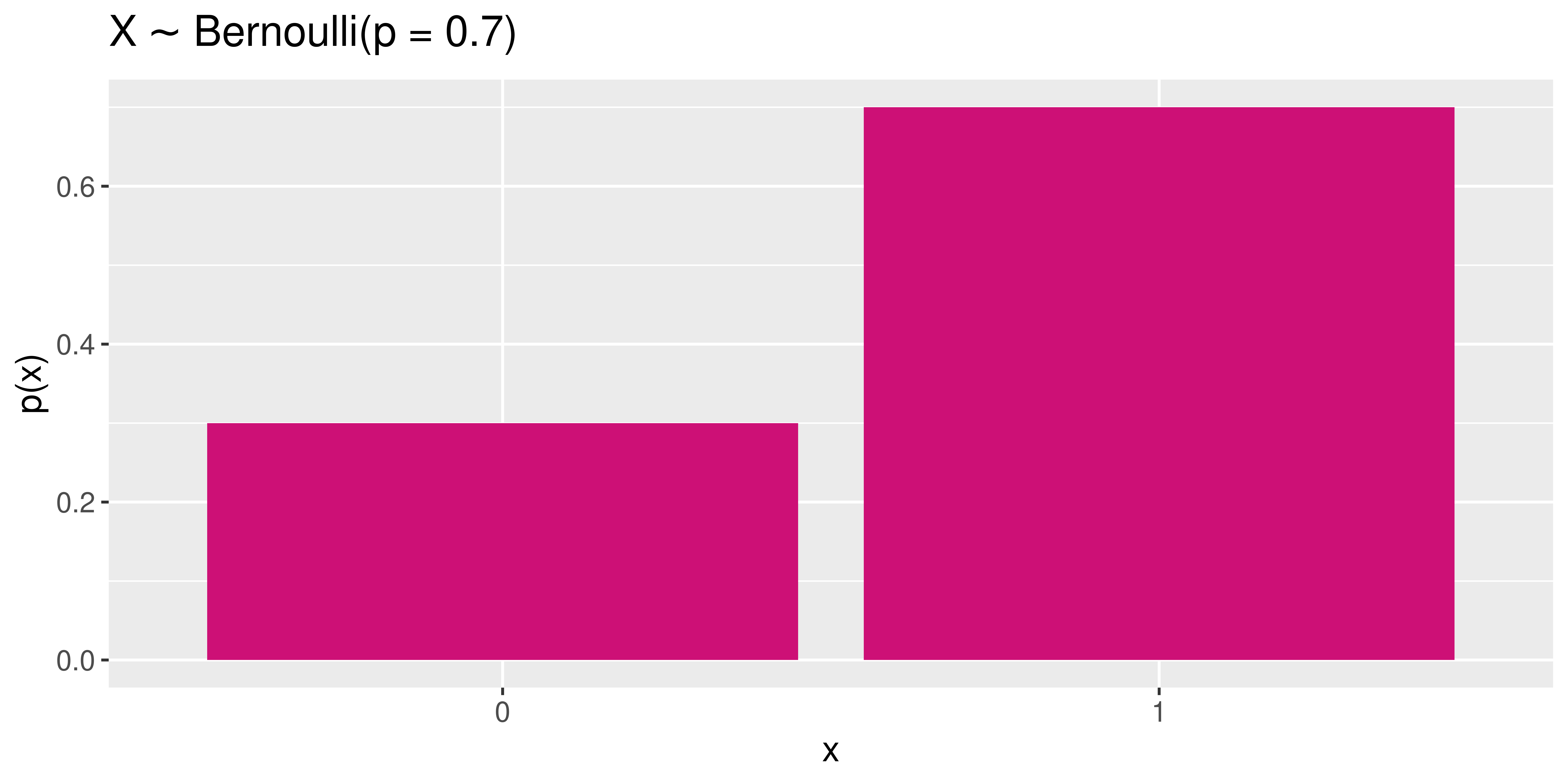
Bernoulli Random Variables
\(X \sim\) Bernoulli \((p)\)
\[\begin{align*}
X= \left\{
\begin{array}{ll}
1 & \mbox{success} \\
0 & \mbox{failure} \\
\end{array}
\right.
\end{align*}\]
Important parameter:
\[
\begin{align*}
p & = \mbox{probability of success} \\
& = P(X = 1)
\end{align*}
\]
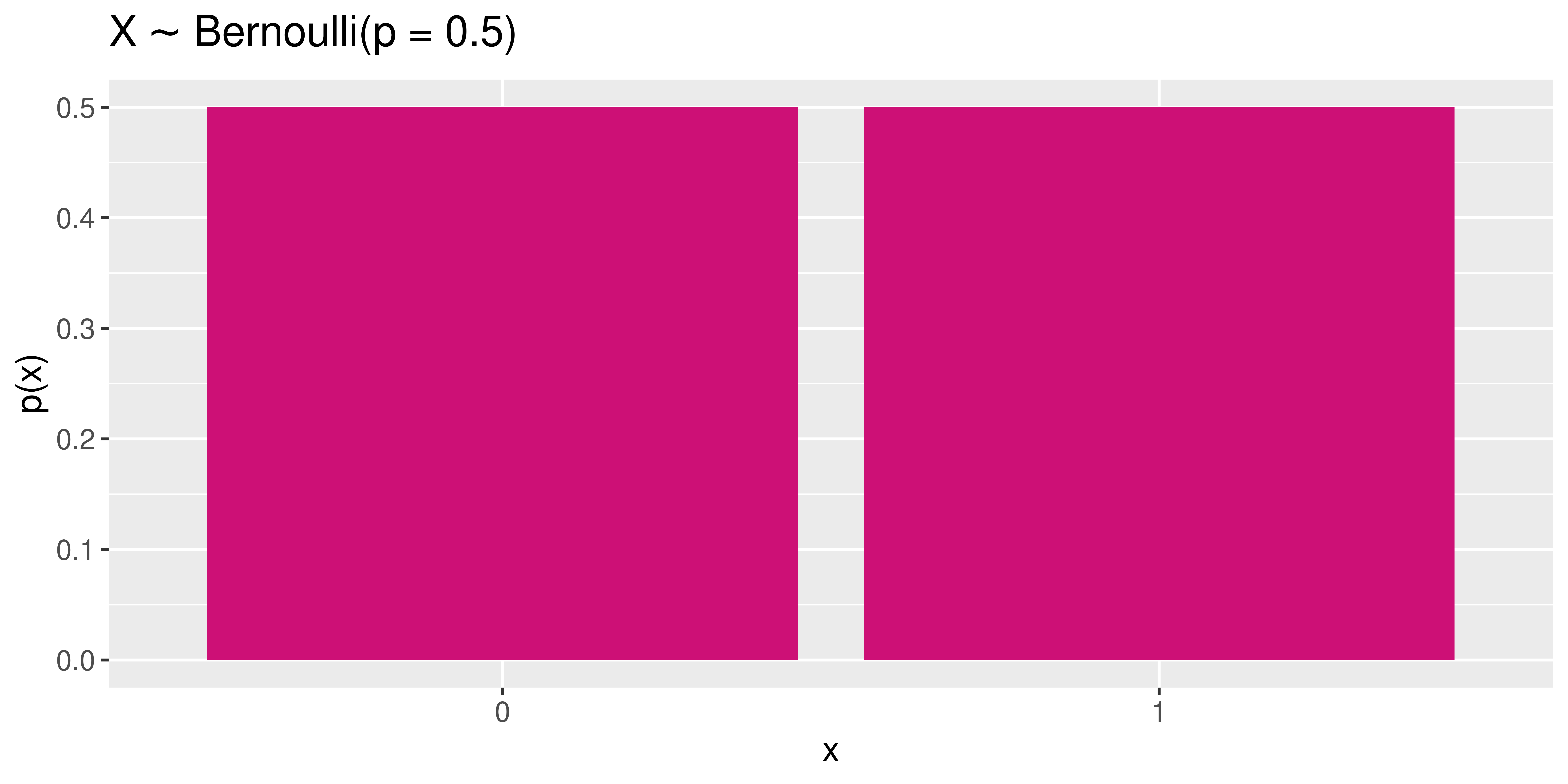
Bernoulli Random Variables
\(X \sim\) Bernoulli \((p = 0.5)\)
\[\begin{align*}
X= \left\{
\begin{array}{ll}
1 & \mbox{success} \\
0 & \mbox{failure} \\
\end{array}
\right.
\end{align*}\]
Bernoulli Random Variables
\(X \sim\) Bernoulli \((p)\)
\[\begin{align*}
X= \left\{
\begin{array}{ll}
1 & \mbox{success} \\
0 & \mbox{failure} \\
\end{array}
\right.
\end{align*}\]
Mean:
\[
\begin{align*}
\mu &= \sum x p(x) \\
& = 1*p + 0*(1 - p) \\
& = p
\end{align*}
\]
Bernoulli Random Variables
\(X \sim\) Bernoulli \((p)\)
\[\begin{align*}
X= \left\{
\begin{array}{ll}
1 & \mbox{success} \\
0 & \mbox{failure} \\
\end{array}
\right.
\end{align*}\]
Standard deviation:
\[
\begin{align*}
\sigma & = \sqrt{ \sum (x - \mu)^2 p(x)} \\
& = \sqrt{(1 - p)^2*p + (0 - p)^2*(1 - p)} \\
& = \sqrt{p(1 - p)}
\end{align*}
\]
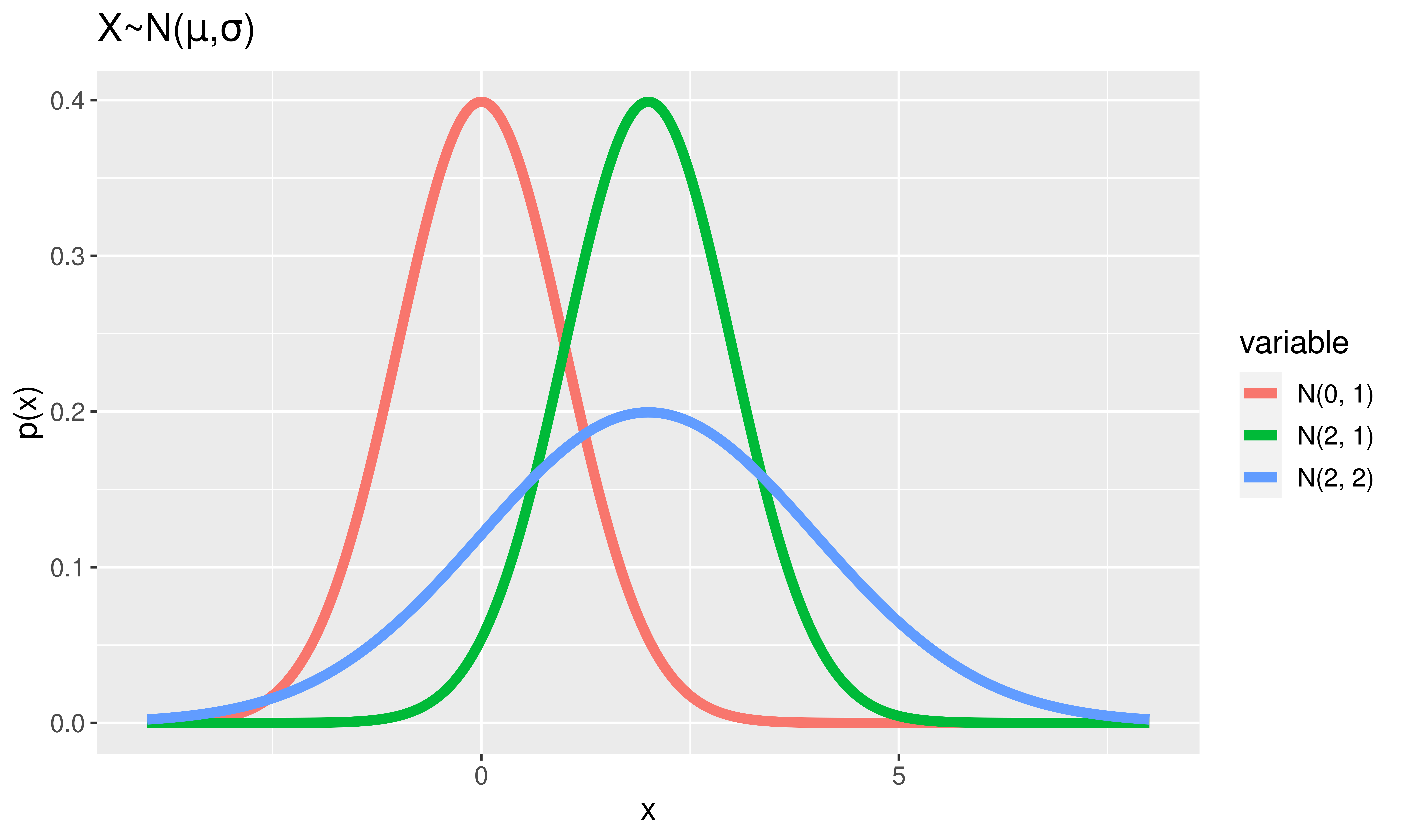
Normal Random Variables
\(X \sim\) Normal \((\mu, \sigma)\)
Distribution:
\[
p(x) = \frac{1}{\sqrt{2\pi \sigma^2}}\exp{\left(-\frac{(x - \mu)^2}{2\sigma^2} \right)}
\] where \(-\infty < x < \infty\)
Normal Random Variables
\(X \sim\) Normal \((\mu, \sigma)\)
Notes:
Area under the curve = 1.
Height \(\approx\) how likely values are to occur
Super special Normal RV:
\(Z \sim\) Normal \((\mu = 0, \sigma = 1)\).
Normal Random Variables
\(X \sim\) Normal \((\mu, \sigma)\)
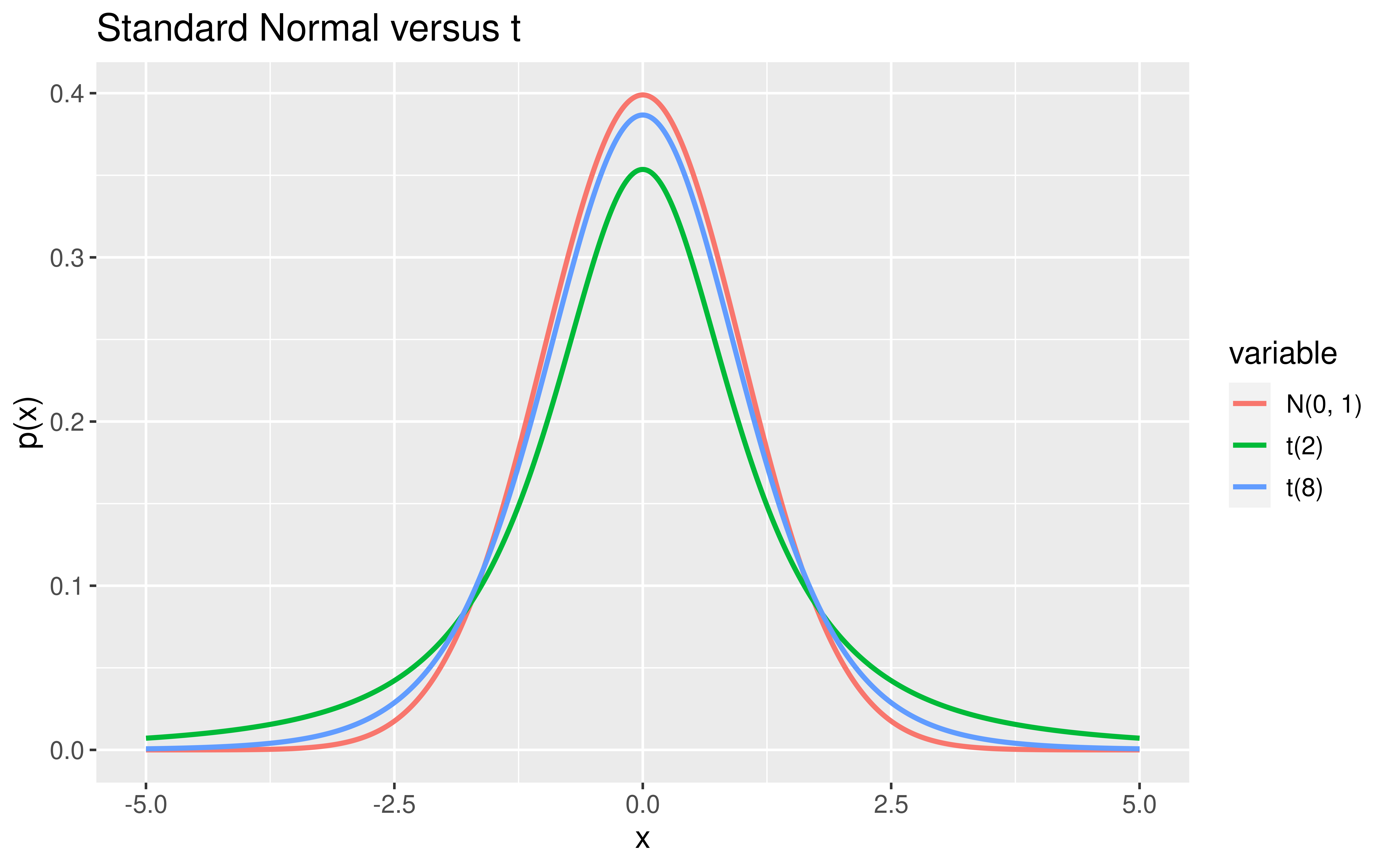
t Random Variables
\(X \sim\) t(df)
Distribution:
\[
p(x) = \frac{\Gamma(\mbox{df} + 1)}{\sqrt{\mbox{df}\pi} \Gamma(2^{-1}\mbox{df})}\left(1 + \frac{x^2}{\mbox{df}} \right)^{-\frac{df + 1}{2}}
\]
where \(-\infty < x < \infty\)
It is time to recast some of the sample statistics we have been exploring as random variables!
Sample Statistics as Random Variables
Here are some of the sample statistics we’ve seen lately:
\(\hat{p}\) = sample proportion of correct receiver guesses out of 329 trials
\(\bar{x}_I - \bar{x}_N\) = difference in sample mean tuition between Ivies and non-Ivies
\(\hat{p}_D - \hat{p}_Y\) = difference in sample improvement proportions between those who swam with dolphins and those who did not
Why are these all random variables?
- But they aren’t Bernoulli random variables, nor Normal random variables, nor t random variables.
“All models are wrong but some are useful.” – George Box
Approximating These Distributions
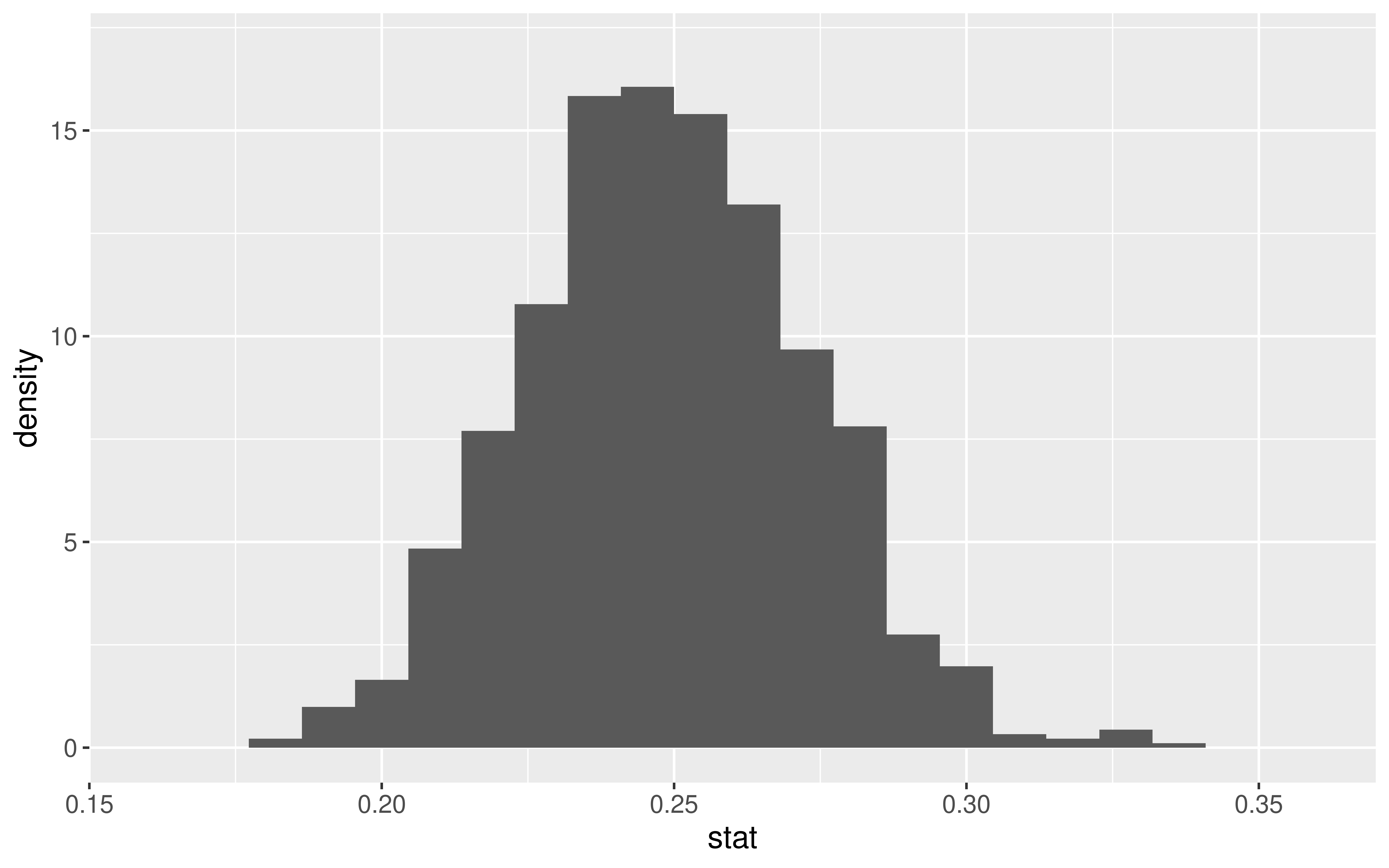
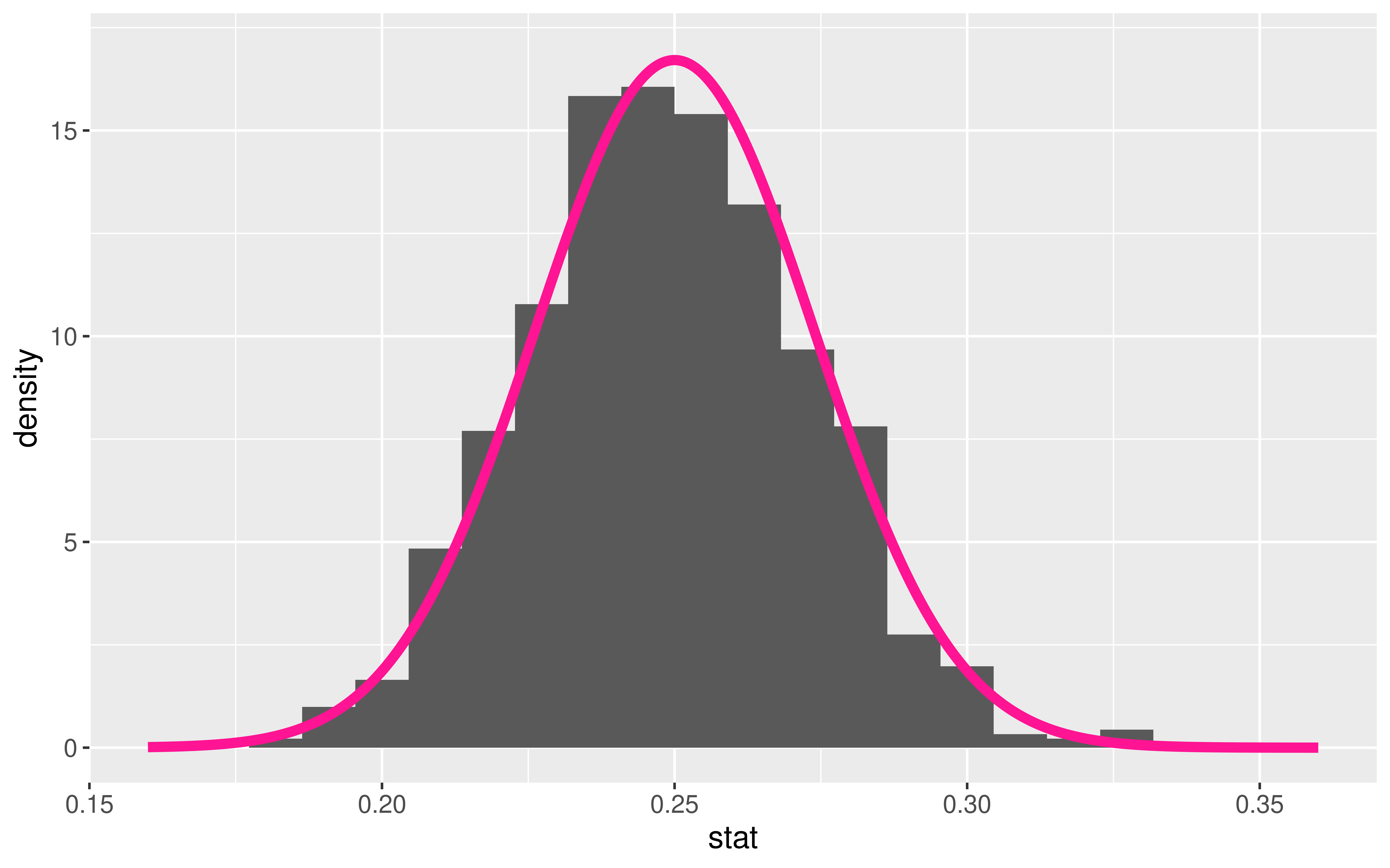
- \(\hat{p}\) = sample proportion of correct receiver guesses out of 329 trials
We generated its Null Distribution:
Which is well approximated by the distribution of a N(0.25, 0.024).
Approximating These Distributions
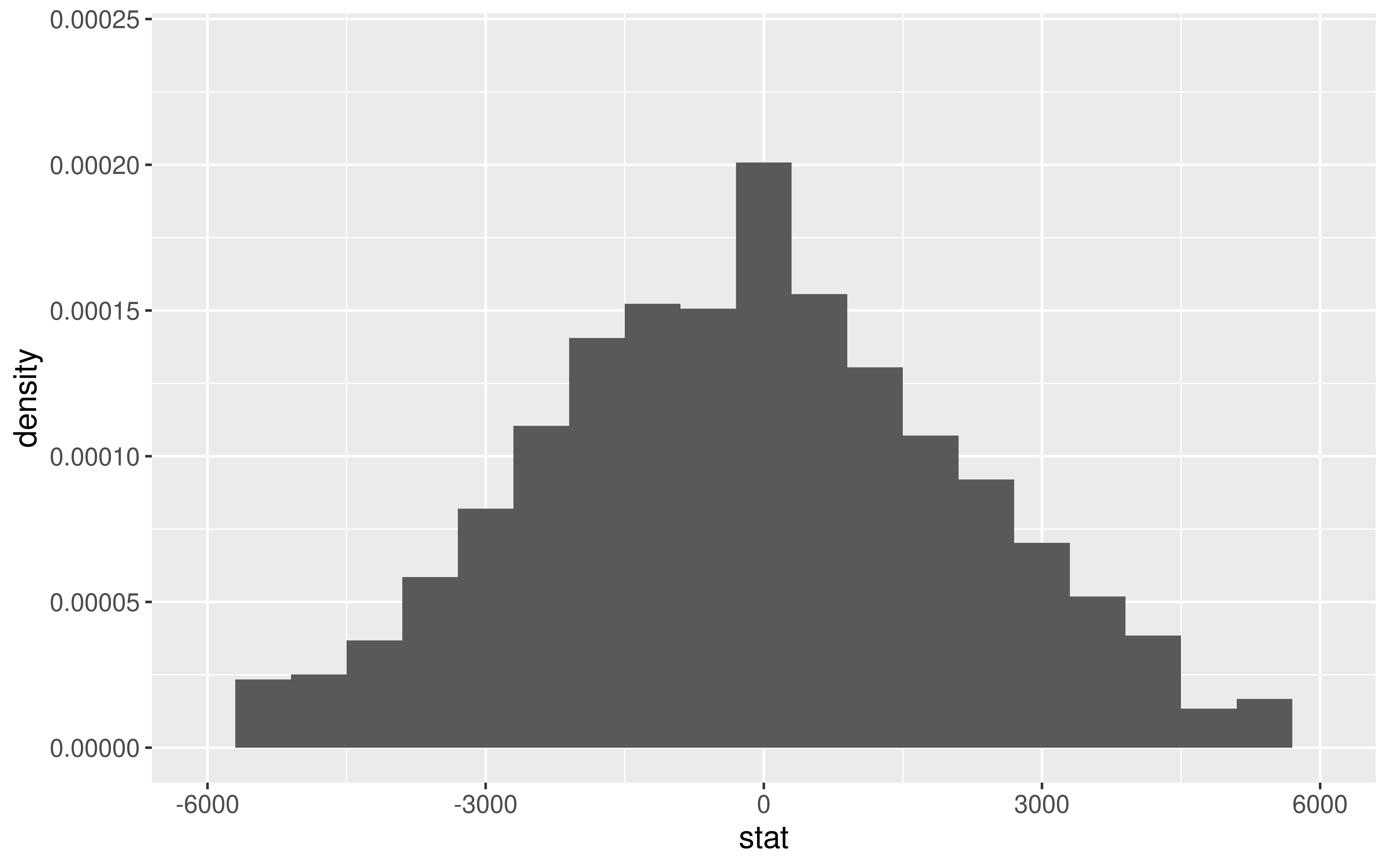
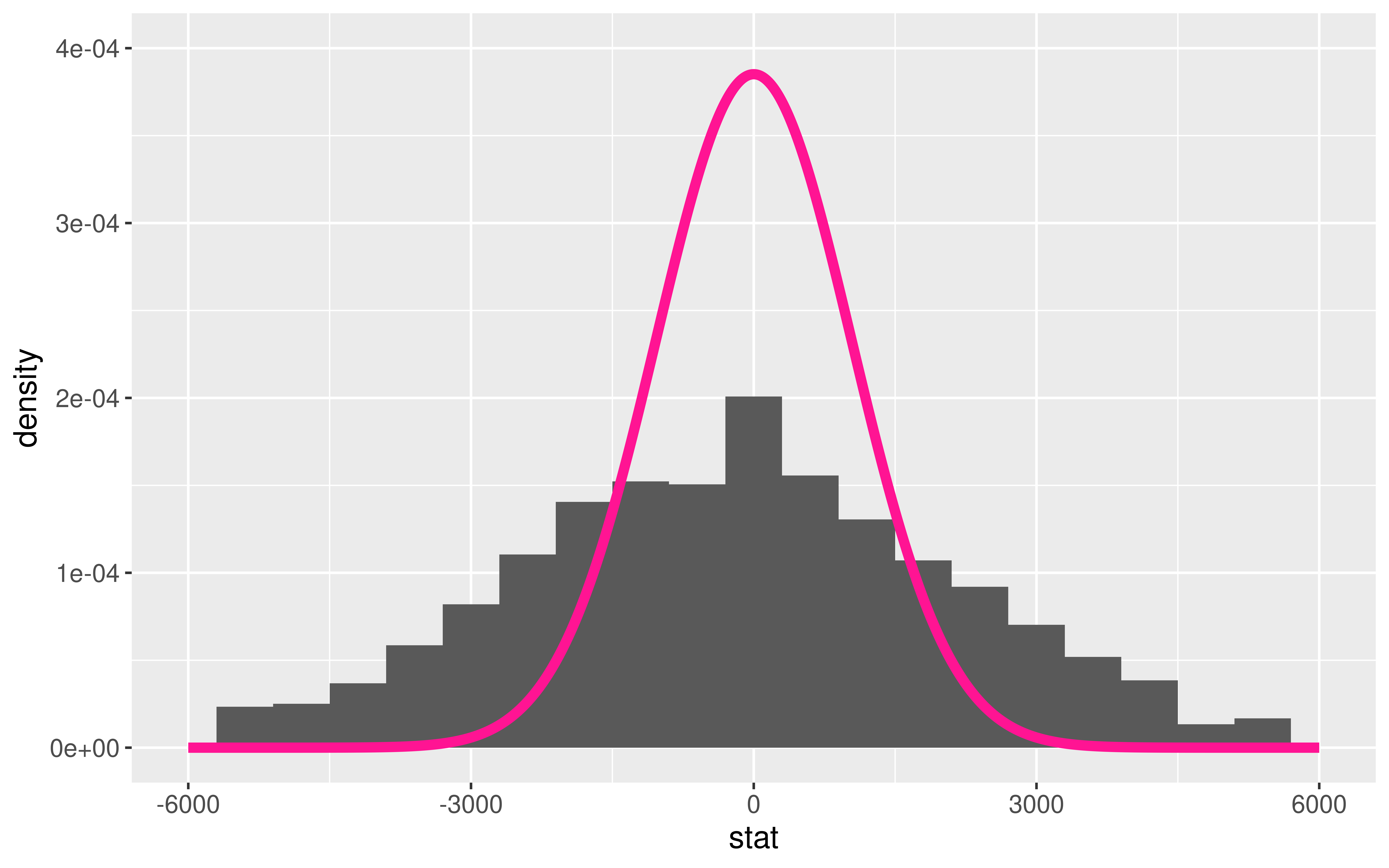
- \(\bar{x}_I - \bar{x}_N\) = difference in sample mean tuition between Ivies and non-Ivies
We generated its Null Distribution:
Which is somewhat approximated by the distribution of a N(0, 1036).
We will learn that a standardized version of the difference in sample means is better approximated by the distribution of a t(df = 7).
Approximating These Distributions
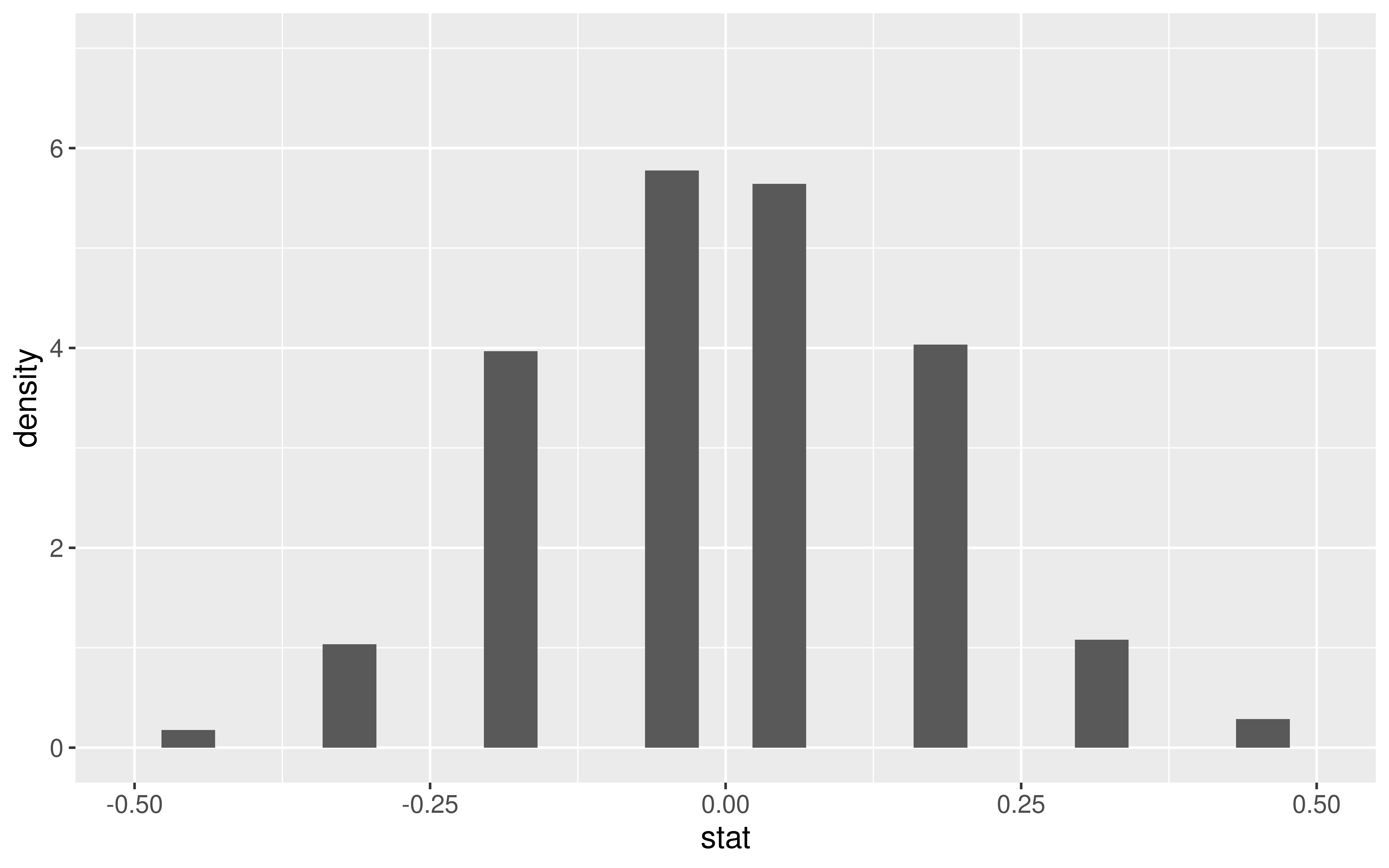
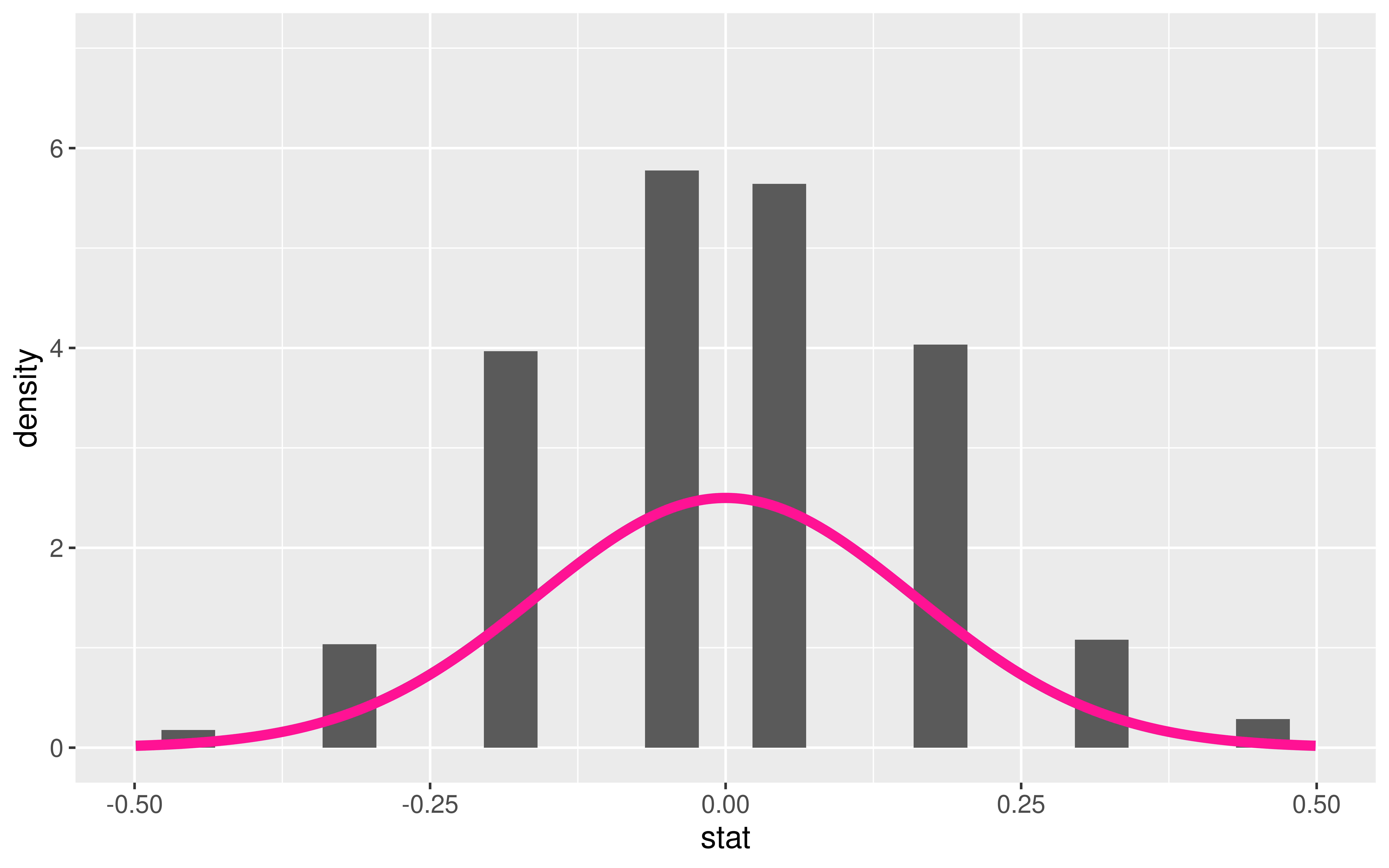
- \(\hat{p}_D - \hat{p}_Y\) = difference in sample improvement proportions between those who swam with dolphins and those who did not
We generated its Null Distribution:
Which is kinda somewhat approximated by the probability function of a N(0, 0.16).
Approximating These Distributions
How do I know which probability function is a good approximation for my sample statistic’s distribution?
Once I have figured out a probability function that approximates the distribution of my sample statistic, how do I use it to do statistical inference?
Central Limit Theorem
Central Limit Theorem (CLT): For random samples and a large sample size \((n)\), the sampling distribution of many sample statistics is approximately normal.
Example: Harvard Trees
Approximating Sampling Distributions
Central Limit Theorem (CLT): For random samples and a large sample size \((n)\), the sampling distribution of many sample statistics is approximately normal.
Example: Harvard Trees
- But which Normal? (What is the value of \(\mu\) and \(\sigma\)?)
Approximating Sampling Distributions
Question: But which normal? (What is the value of \(\mu\) and \(\sigma\)?)
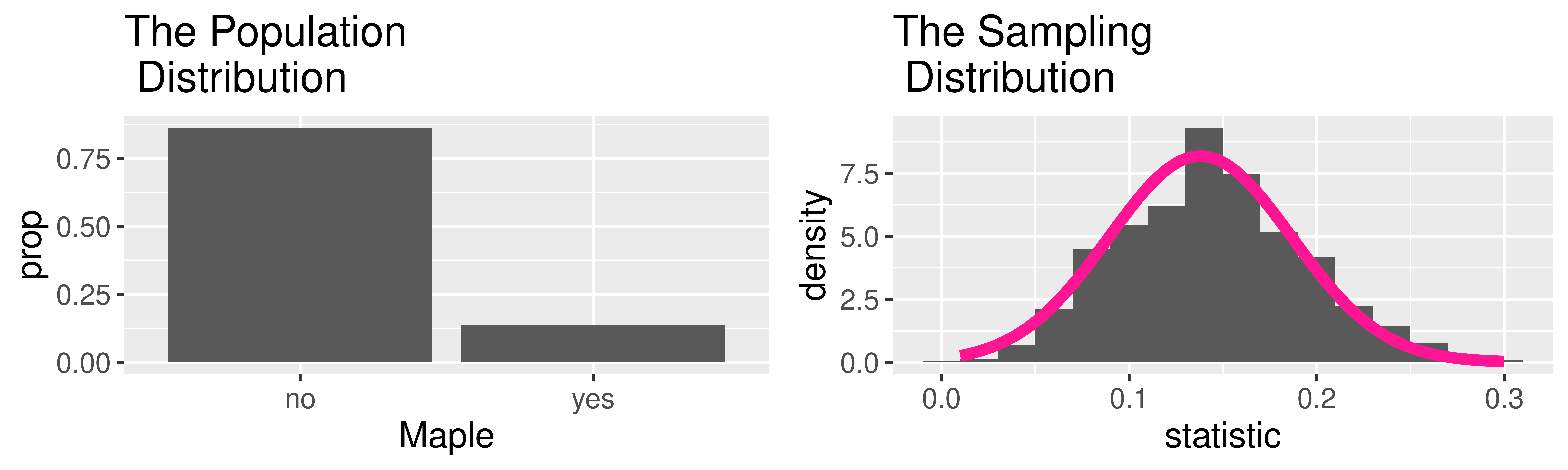
Approximating the Sampling Distribution of a Sample Proportion
CLT says: For large \(n\) (At least 10 successes and 10 failures),
\[
\hat{p} \sim N \left(p, \sqrt{\frac{p(1-p)}{n}} \right)
\]
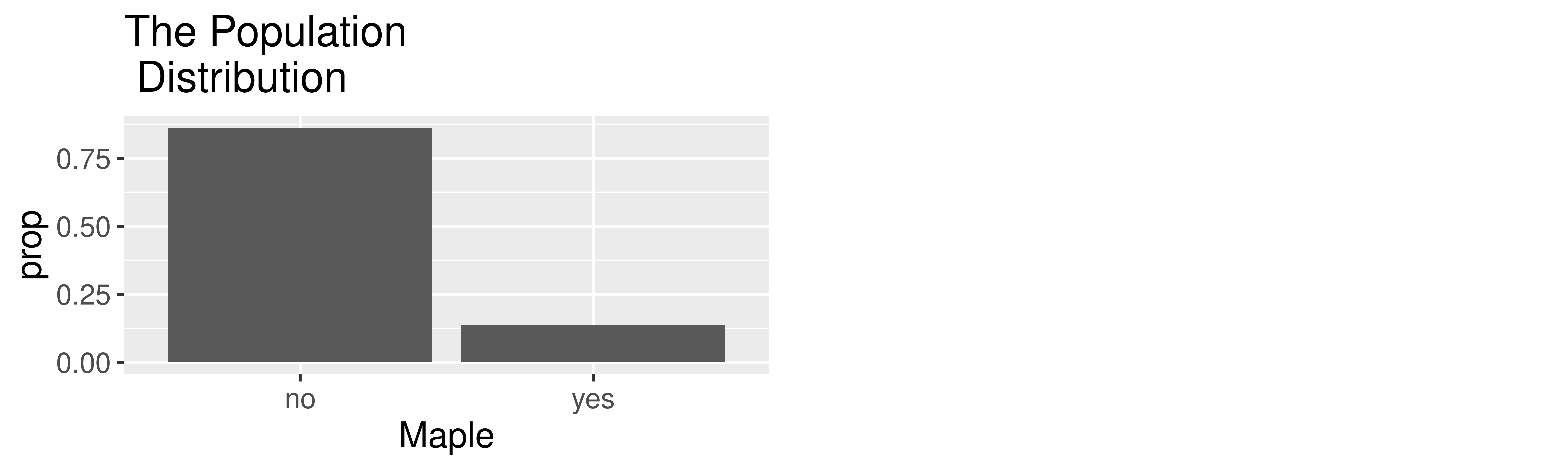
Example: Maples at Harvard
\[
\hat{p} \sim N \left(0.138, \sqrt{\frac{0.138(1-0.138)}{50}} \right)
\]
NOTE: Can plug in the true parameter here because we had data on the whole population.
Approximating the Sampling Distribution of a Sample Proportion
Question: What do we do when we don’t have access to the whole population?
Have:
\[
\hat{p} \sim N \left(p, \sqrt{\frac{p(1-p)}{n}} \right)
\]
Answer: We will have to estimate the SE.
Approximating the Sampling Distribution of a Sample Mean
There is a version of the CLT for many of our sample statistics.
For the sample mean, the CLT says: For large \(n\) (At least 30 observations),
\[
\bar{x} \sim N \left(\mu, \frac{\sigma}{\sqrt{n}} \right)
\]
Next time: Use the approximate distribution of the sample statistic (given by the CLT) to construct confidence intervals and to conduct hypothesis tests!
Reminders:
- No sections or wrap-ups during Thanksgiving Week.
- OH schedule for Thanksgiving Week: