Theory-Based Inference

Kelly McConville

Stat 100
Week 12 | Fall 2023

Announcements

• No sections or wrap-ups this week.
• P-Set 8 is due next Tues (5pm) but try to get most of your questions answered before Thanksgiving Break!
• No new p-set or lecture quiz this week.
• OH schedule for Thanksgiving Week:
  • Sun, Nov 19th - Tues, Nov 21st: Happening with some modifications
  • No OHs Wed, Nov 22nd - Sun, Nov 26th!

Goals for Today

• A bit of thanks.

• Learn theory-based statistical inference methods.

• Introduce a new group of test statistics based on z-scores.

• Generalize the SE method confidence interval formula.

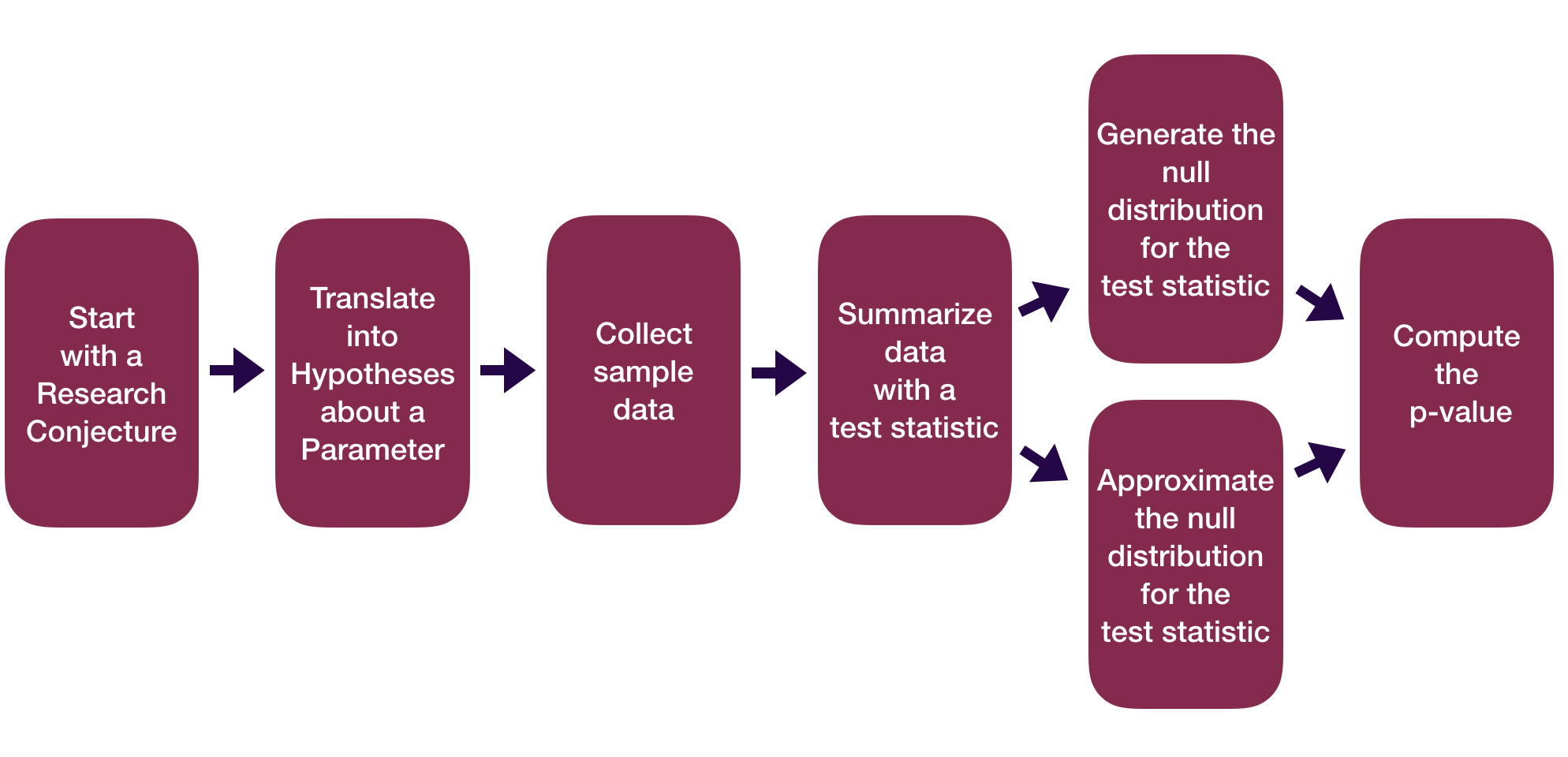
Statistical Inference Zoom Out – Estimation

Statistical Inference Zoom Out – Testing

Sample Statistics as Random Variables

• Sample statistics can be recast as random variables.

• Need to figure out what random variable is a good approximation for our sample statistic.

  • Then use the properties of that random variable to do inference.

• Sometimes it is easier to find a good random variable approximation if we standardize our sample statistic first.

Z-scores

• All of our test statistics so far have been sample statistics.

• Another commonly used test statistic takes the form of a z-score:

\[ \mbox{Z-score} = \frac{X - \mu}{\sigma} \]

• Standardized version of the sample statistic.

• Z-score measures how many standard deviations the sample statistic is away from its mean.

Z-score Example

• \(\hat{p}\) = proportion of Maples in a sample of 50 trees

\[ \hat{p} \sim N \left(0.138, 0.049 \right) \]

• Suppose we have a sample where \(\hat{p} = 0.05\). Then the z-score would be:

\[ \mbox{Z-score} = \frac{0.05 - 0.138}{0.049} = -1.8 \]

Z-score Test Statistics

• A Z-score test statistic is one where we take our original sample statistic and convert it to a Z-score:

\[ \mbox{Z-score test statistic} = \frac{\mbox{statistic} - \mu}{\sigma} \]

• Allows us to quickly (but roughly) classify results as unusual or not.
  • \(|\) Z-score \(|\) > 2 → results are unusual/p-value will be smallish
• Commonly used because if the sample statistic \(\sim N(\mu, \sigma)\), then

\[ \mbox{Z-score test statistic} = \frac{\mbox{statistic} - \mu}{\sigma} \sim N(0, 1) \]

Let’s consider theory-based inference for a population proportion.

Statistical Inference Zoom Out – Estimation

Statistical Inference Zoom Out – Testing

Inference for a Single Proportion – Testing

Let’s consider conducting a hypothesis test for a single proportion: \(p\)

Need:

• Hypotheses
  • Same as with the simulation-based methods
• Test statistic and its null distribution
  • Use a z-score test statistic and a standard normal distribution
• P-value
  • Compute from the standard normal distribution directly

Inference for a Single Proportion – Testing

Let’s consider conducting a hypothesis test for a single proportion: \(p\)

\(H_o: p = p_o\) where \(p_o\) = null value and \(H_a: p > p_o\) or \(H_a: p < p_o\) or \(H_a: p \neq p_o\)

By the CLT, under \(H_o\):

\[ \hat{p} \sim N \left(p_o, \sqrt{\frac{p_o(1-p_o)}{n}} \right) \]

Z-score test statistic:

\[ Z = \frac{\hat{p} - p_o}{\sqrt{\frac{p_o(1-p_o)}{n}}} \]

Use \(N(0, 1)\) to find the p-value once you have computed the test statistic.

Inference for a Single Proportion – Testing

Let’s consider conducting a hypothesis test for a single proportion: \(p\)

Example: Bern and Honorton’s (1994) extrasensory perception (ESP) studies

# Construct data frame of sample results
esp <- data.frame(guess = c(rep("correct", 106),
                            rep("incorrect", 329 - 106)))

Inference for a Single Proportion – Testing

Let’s consider conducting a hypothesis test for a single proportion: \(p\)

Example: Bern and Honorton’s (1994) extrasensory perception (ESP) studies

library(infer)
# Compute observed test statistic
test_stat <- esp %>%
  specify(response = guess,
          success = "correct") %>%
  hypothesize(null = "point", p = 0.25) %>%  
  calculate(stat = "z")
test_stat

Response: guess (factor)
Null Hypothesis: point
# A tibble: 1 × 1
   stat
  <dbl>
1  3.02

# Use N(0,1) to find p-value
pnorm(q = test_stat$stat, mean = 0, sd = 1,
      lower.tail = FALSE)

[1] 0.001247763

# Or 
1 - pnorm(q = test_stat$stat,
          mean = 0, sd = 1)

[1] 0.001247763

prop_test(esp, response = guess, success = "correct", p = 0.25,
          z = TRUE, alternative = "greater")

# A tibble: 1 × 3
  statistic p_value alternative
      <dbl>   <dbl> <chr>      
1      3.02 0.00125 greater    

Note: There is also a base R function called prop.test() but its arguments are different.

Theory-Based Confidence Intervals

Suppose statistic \(\sim N(\mu = \mbox{parameter}, \sigma = SE)\).

95% CI for parameter:

\[ \mbox{statistic} \pm 2 SE \]

Can generalize this formula!

P% CI for parameter:

\[ \mbox{statistic} \pm z^* SE \]

# Find z-star
qnorm(p = 0.975, mean = 0, sd = 1)

[1] 1.959964

qnorm(p = 0.95, mean = 0, sd = 1)

[1] 1.644854

Theory-Based CIs in Action

Let’s consider constructing a confidence interval for a single proportion: \(p\)

By the CLT,

\[ \hat{p} \sim N \left(p, \sqrt{\frac{p(1-p)}{n}} \right) \]

P% CI for parameter:

\[\begin{align*} \mbox{statistic} \pm z^* SE \end{align*}\]

Theory-Based CIs in Action

Example: Bern and Honorton’s (1994) extrasensory perception (ESP) studies

# Use probability model to approximate null distribution
prop_test(esp, response = guess, success = "correct", 
          z = TRUE, conf_int = TRUE, conf_level = 0.95)

# A tibble: 1 × 5
  statistic  p_value alternative lower_ci upper_ci
      <dbl>    <dbl> <chr>          <dbl>    <dbl>
1     -6.45 1.12e-10 two.sided      0.274    0.374

• Don’t use the reported test statistic and p-value!

Theory-Based CIs

P% CI for parameter:

\[ \mbox{statistic} \pm z^* SE \]

Notes:

• Didn’t construct the bootstrap distribution.

• Need to check that \(n\) is large and that the sample is random/representative.

  • Condition depends on what parameter you are conducting inference for.

count(esp, guess)

      guess   n
1   correct 106
2 incorrect 223

• Interpretation of the CI doesn’t change.

• For some parameters, the critical value comes from a \(t\) distribution.

• Now we have a formula for the Margin of Error.

  • That will prove useful for sample size calculations.

Now let’s explore how to do inference for a single mean.

Inference for a Single Mean

Example: Are lakes in Florida more acidic or alkaline? The pH of a liquid is the measure of its acidity or alkalinity where pure water has a pH of 7, a pH greater than 7 is alkaline and a pH less than 7 is acidic. The following dataset contains observations on a sample of 53 lakes in Florida.

library(tidyverse)
FloridaLakes <- read_csv("https://www.lock5stat.com/datasets1e/FloridaLakes.csv")

Cases:

Variable of interest:

Parameter of interest:

Hypotheses:

Inference for a Single Mean

Let’s consider conducting a hypothesis test for a single mean: \(\mu\)

Need:

• Hypotheses
  • Same as with the simulation-based methods
• Test statistic and its null distribution
  • Use a z-score test statistic and a t distribution
• P-value
  • Compute from the t distribution directly

Inference for a Single Mean

Let’s consider conducting a hypothesis test for a single mean: \(\mu\)

\(H_o: \mu = \mu_o\) where \(\mu_o\) = null value

\(H_a: \mu > \mu_o\) or \(H_a: \mu < \mu_o\) or \(H_a: \mu \neq \mu_o\)

By the CLT, under \(H_o\):

\[ \bar{x} \sim N \left(\mu_o, \frac{\sigma}{\sqrt{n}} \right) \]

Z-score test statistic:

\[ Z = \frac{\bar{x} - \mu_o}{\frac{\sigma}{\sqrt{n}}} \]

• Problem: Don’t know \(\sigma\): the population standard deviation of our response variable!

Inference for a Single Mean

Z-score test statistic:

\[ t = \frac{\bar{x} - \mu_o}{\frac{s}{\sqrt{n}}} \]

• Problem: Don’t know \(\sigma\): the population standard deviation of our response variable!
  • For our example, \(\sigma\) would be the standard deviation of the Ph level for all lakes in Florida.
• Solution: Plug in \(s\): the sample standard deviation of our response variable!
  • For our example, \(s\) would be the standard deviation of the Ph level for the sampled lakes in Florida.
• Use \(t(\mbox{df} = n - 1)\) to find the p-value

Inference for a Single Mean

library(infer)

#Compute obs stat
t_obs <- FloridaLakes %>%
  specify(response = pH) %>%
  hypothesize(null = "point", mu = 7) %>%  
  calculate(stat = "t")
t_obs

Response: pH (numeric)
Null Hypothesis: point
# A tibble: 1 × 1
   stat
  <dbl>
1 -2.31

# Generate null distribution
null_dist <- FloridaLakes %>%
 specify(response = pH) %>%
 hypothesize(null = "point", mu = 7) %>%
 generate(reps = 1000, type = "bootstrap") %>%
 calculate(stat = "t")

Why are we using type = "bootstrap" when constructing a null distribution?!

Inference for a Single Mean

What probability function is a good approximation to the null distribution?

null_dist %>%
  visualize(bins = 30) +
  geom_vline(xintercept = t_obs$stat,
             color = "deeppink",
             size = 2) +
  geom_vline(xintercept = abs(t_obs$stat),
             color = "deeppink", 
             size = 2)

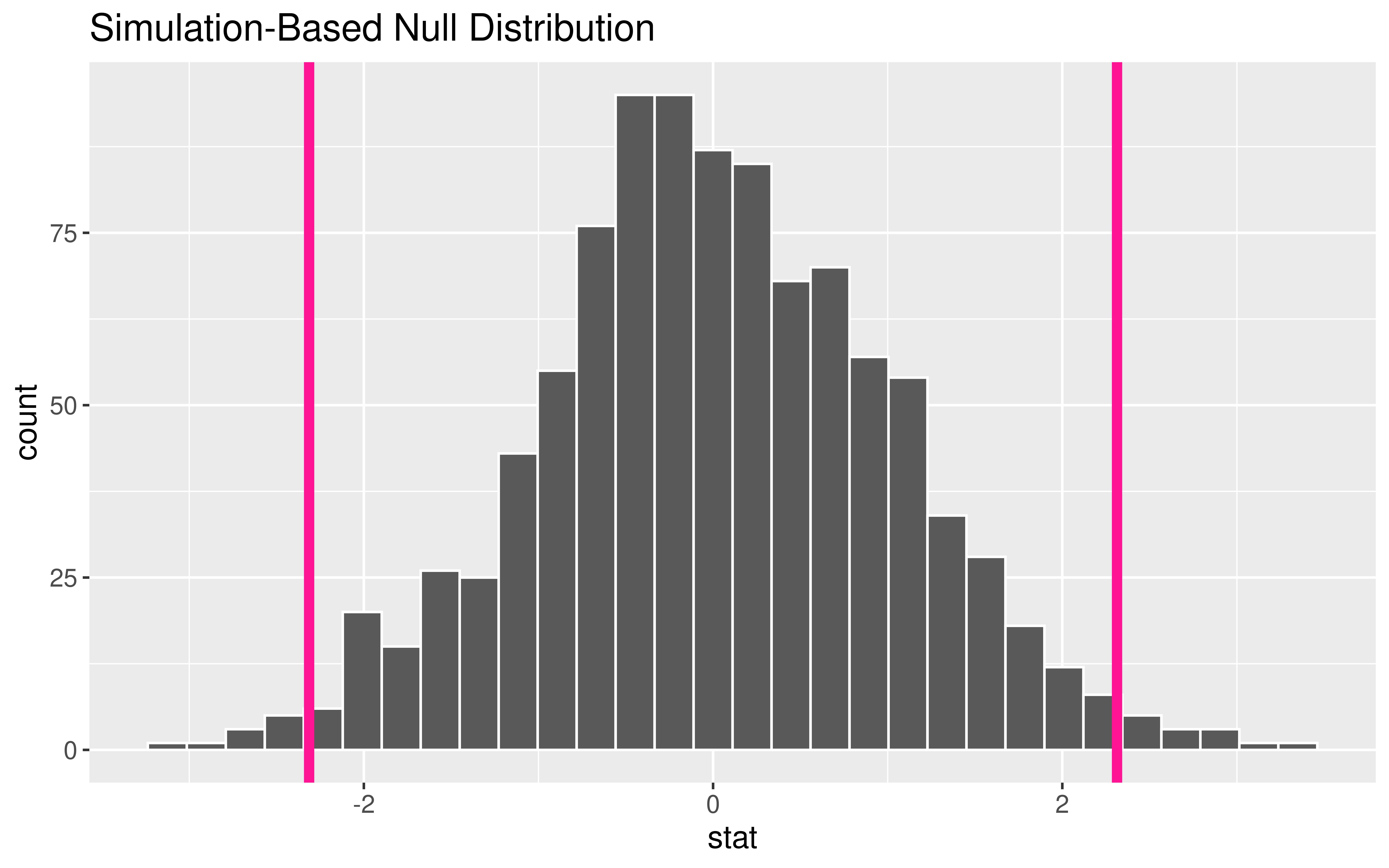
Inference for a Single Mean

What probability function is a good approximation to the null distribution?

null_dist %>%
  visualize(bins = 30, method = "both",
            dens_color = "orange") +
  geom_vline(xintercept = t_obs$stat,
             color = "deeppink",
             size = 2) +
  geom_vline(xintercept = abs(t_obs$stat),
             color = "deeppink", 
             size = 2)

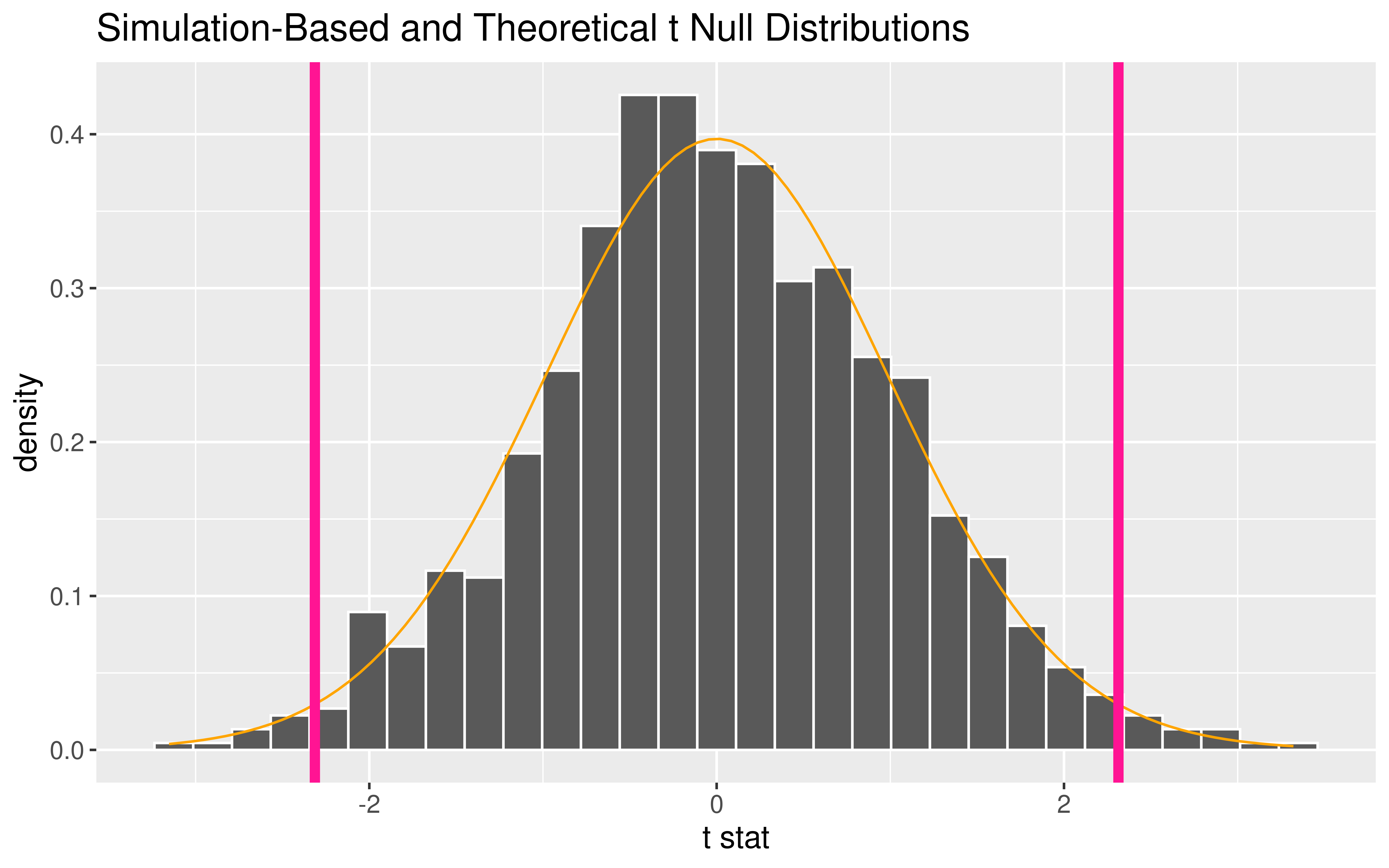
P-value options

P-value using the generated null distribution:

pvalue <- null_dist %>%
  get_p_value(obs_stat = t_obs,
              direction = "both")
pvalue

# A tibble: 1 × 1
  p_value
    <dbl>
1   0.022

P-value using an approximate probability function:

# Using t distribution
pt(q = t_obs$stat, df = 52)*2

         t 
0.02468707 

Do-it-all function:

t_test(FloridaLakes, response = pH, mu = 7,
       alternative = "two-sided")

# A tibble: 1 × 7
  statistic  t_df p_value alternative estimate lower_ci upper_ci
      <dbl> <dbl>   <dbl> <chr>          <dbl>    <dbl>    <dbl>
1     -2.31    52  0.0247 two.sided       6.59     6.24     6.95

Statistical Inference using Probability Models

• We went through theory-based inference for \(p\) and for \(\mu\).

• There are similar results for other parameters. But the specific named random variable may change!

  • Will extend beyond inference for 1 variable next time.

Have a lovely Thanksgiving Break everyone!

Reminders:

• No sections or wrap-ups this week.
• P-Set 8 is due next Tues (5pm) but try to get most of your questions answered before Thanksgiving Break!
• No new p-set or lecture quiz this week.
• OH schedule for Thanksgiving Week:
  • Sun, Nov 19th - Tues, Nov 21st: Happening with some modifications
  • No OHs Wed, Nov 22nd - Sun, Nov 26th!