Should \(x_2\) be in the model that already contains \(x_1\) and \(x_3\)? Also often asked as “Controlling for \(x_1\) and \(x_3\), is there evidence that \(x_2\) has a relationship with \(y\)?”
After controlling for the other explanatory variables, what is the range of plausible values for \(\beta_3\) (which summarizes the relationship between \(y\) and \(x_3\))?
While \(\hat{y}\) is a point estimate for \(y\), can we also get an interval estimate for \(y\)? In other words, can we get a range of plausible predictions for \(y\)?
She posted all her data and code to GitHub and I did some light wrangling so that we could answer the question:
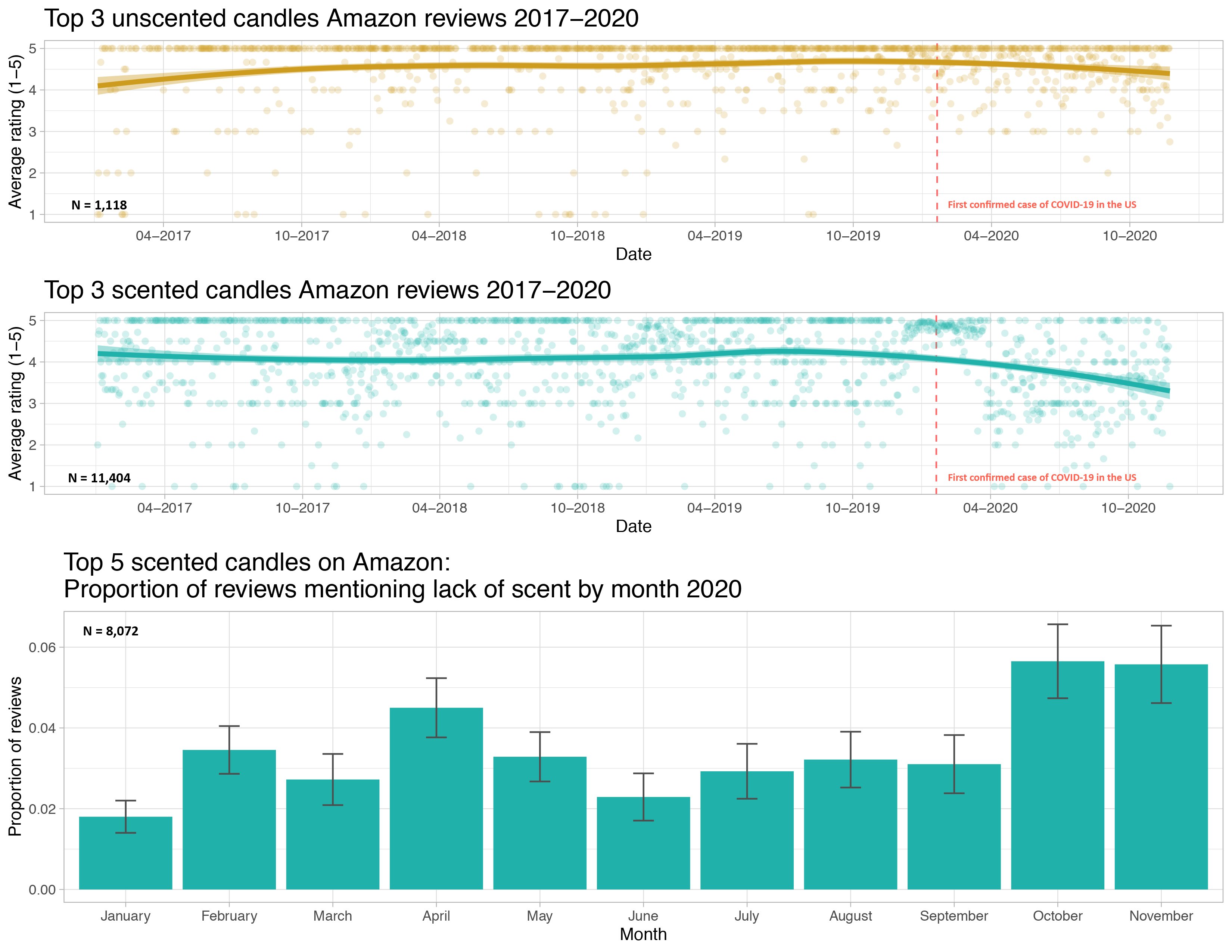
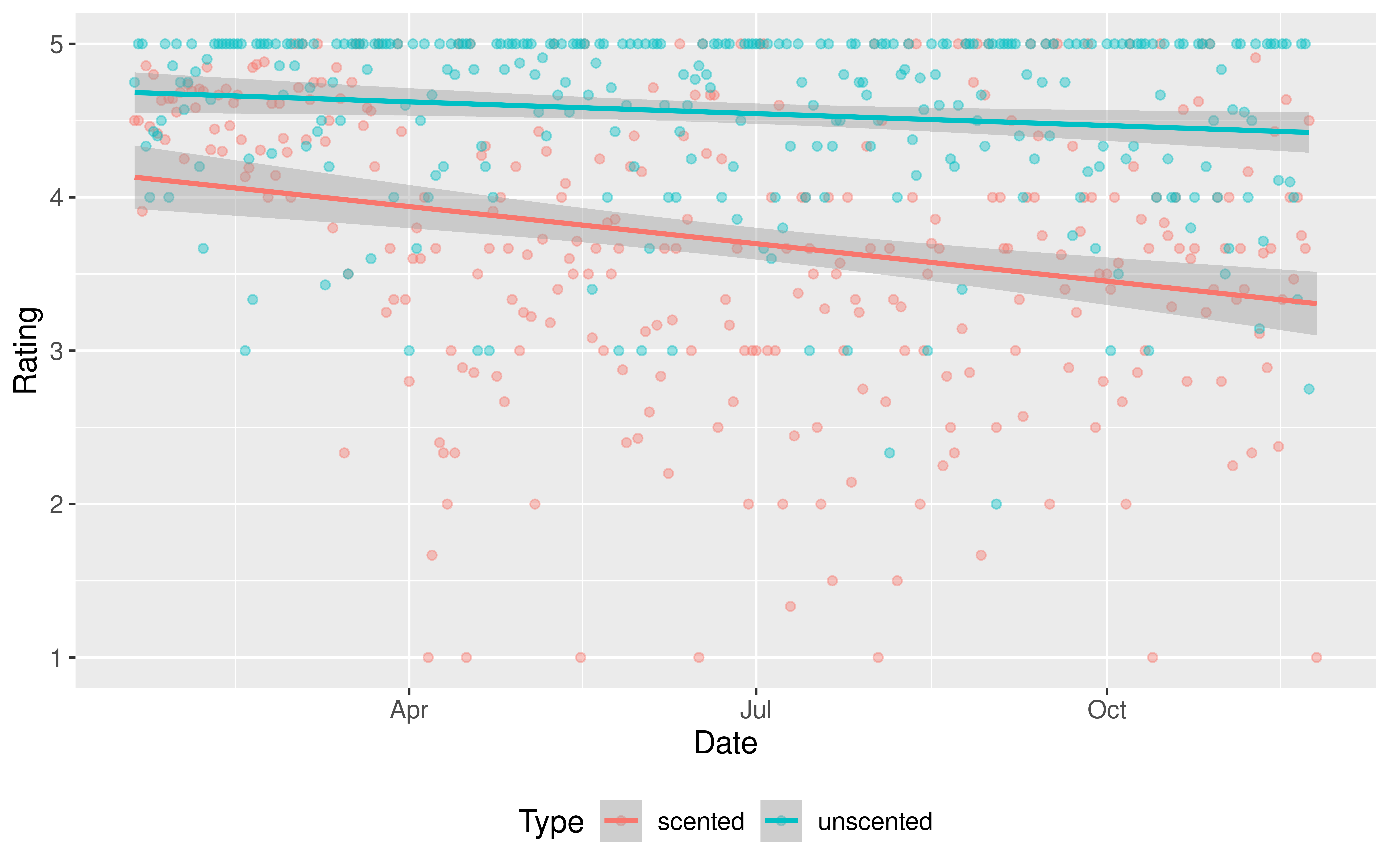
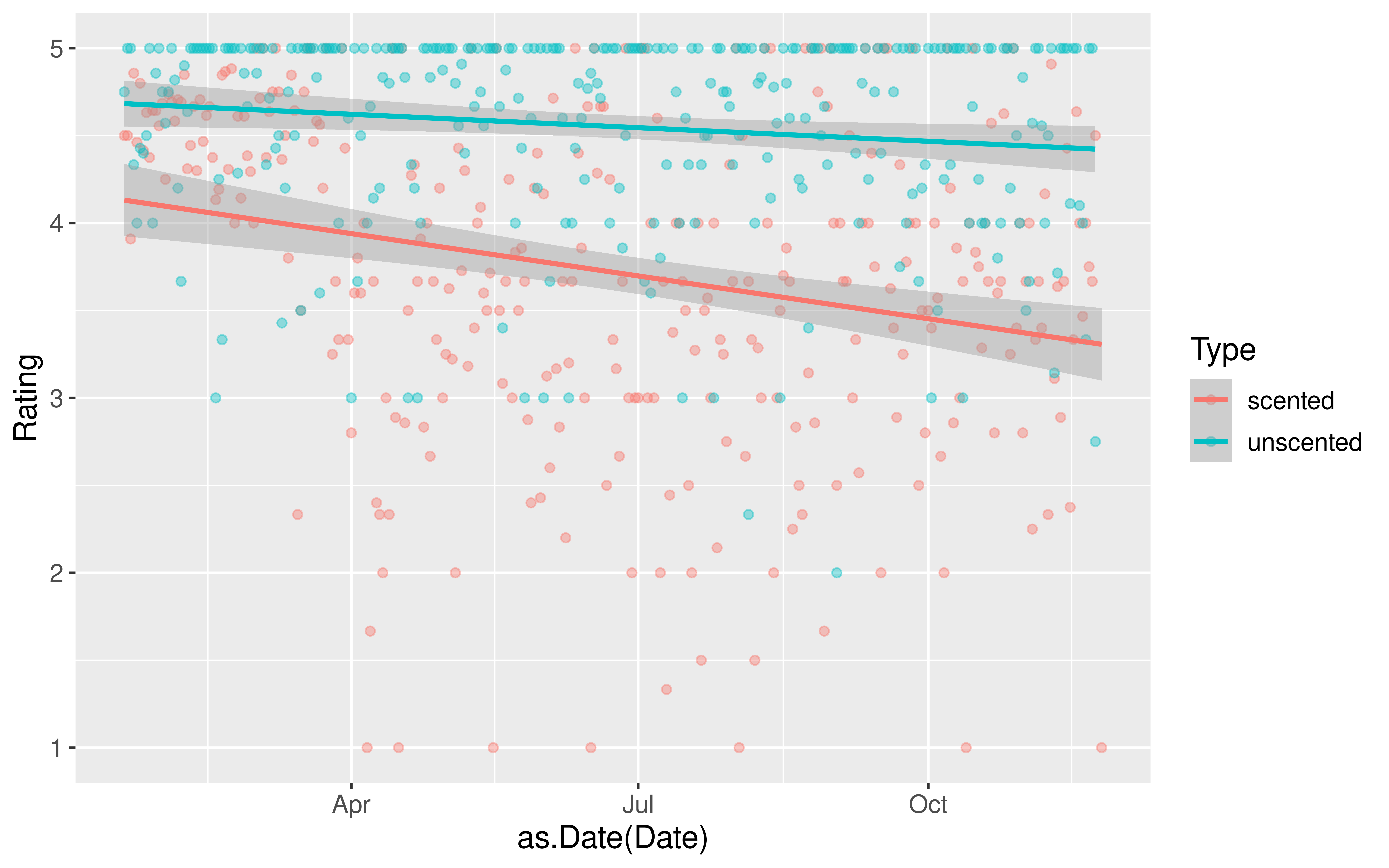
Do we have evidence that early in the pandemic the association between time and Amazon rating varies by whether or not a candle is scented and in particular, that scented candles have a steeper decline in ratings over time?
In other words, do we have evidence that we should allow the slopes to vary?
\[
H_o: \beta_j = 0 \quad \mbox{assuming all other predictors are in the model}
\]\[
H_a: \beta_j \neq 0 \quad \mbox{assuming all other predictors are in the model}
\]
Hypothesis Testing
Question: What tests is get_regression_table() conducting?
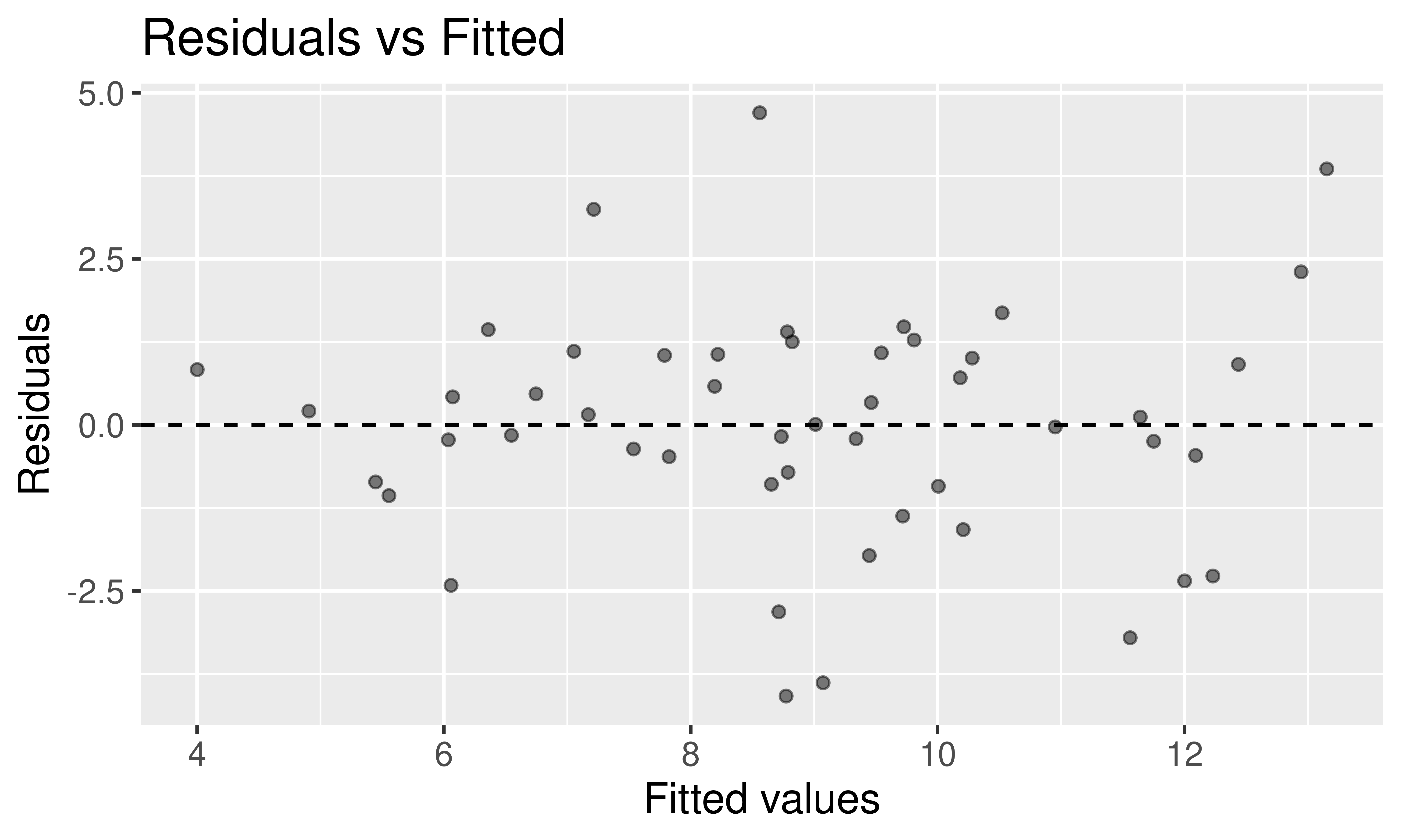
mod <-lm(Rating ~ Date + Type, data = all)get_regression_table(mod)
\[
H_o: \beta_2 = 0 \quad \mbox{given Date is already in the model}
\]\[
H_a: \beta_2 \neq 0 \quad \mbox{given Date is already in the model}
\]
Hypothesis Testing
Question: What tests is get_regression_table() conducting?
In General:
\[
H_o: \beta_j = 0 \quad \mbox{assuming all other predictors are in the model}
\]\[
H_a: \beta_j \neq 0 \quad \mbox{assuming all other predictors are in the model}
\]
Test Statistic: Let \(p\) = number of explanatory variables.
\[
t = \frac{\hat{\beta}_j - 0}{SE(\hat{\beta}_j)} \sim t(df = n - p)
\]
when \(H_o\) is true and the model assumptions are met.
There is evidence that including whether or not the candle is scented adds useful information to the linear regression model for Amazon ratings that already controls for date.
Example
Do we have evidence that early in the pandemic the association between time and Amazon rating varies by whether or not a candle is scented and in particular, that scented candles have a steeper decline in ratings over time?
Do we have evidence that early in the pandemic the association between time and Amazon rating varies by whether or not a candle is scented and in particular, that scented candles have a steeper decline in ratings over time?
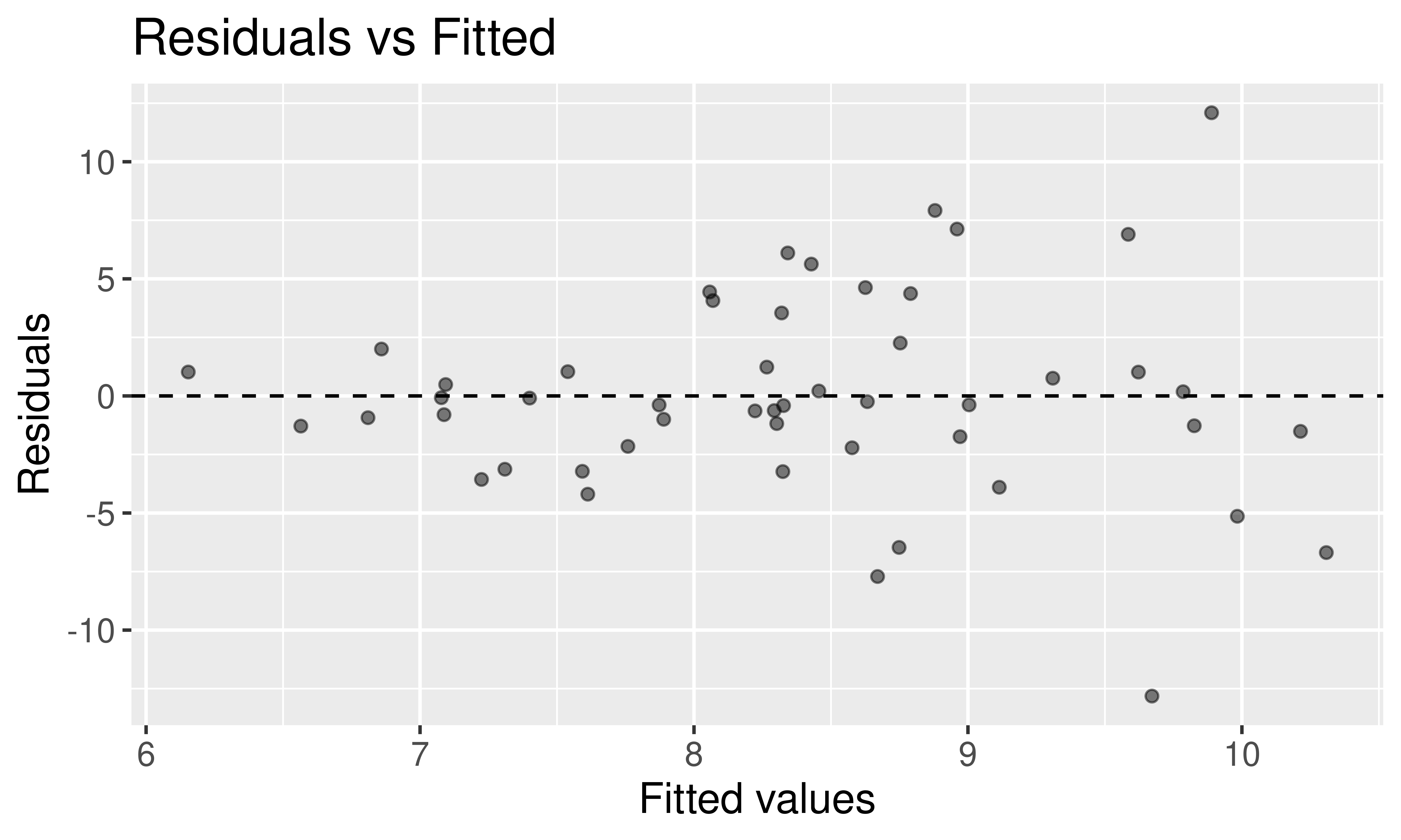
mod <-lm(Rating ~ Date * Type, data = all)get_regression_table(mod)
Now let’s shift our focus to estimation and prediction!
Estimation
Typical Inferential Question:
After controlling for the other explanatory variables, what is the range of plausible values for \(\beta_j\) (which summarizes the relationship between \(y\) and \(x_j\))?
While \(\hat{y}\) is a point estimate for \(y\), can we also get an interval estimate for \(y\)? In other words, can we get a range of plausible predictions for \(y\)?
Two Types of Predictions
Confidence Interval for the Mean Response
→ Defined at given values of the explanatory variables
→ Estimates the average response
→ Centered at \(\hat{y}\)
→ Smaller SE
Prediction Interval for an Individual Response
→ Defined at given values of the explanatory variables
→ Predicts the response of a single, new observation
→ Centered at \(\hat{y}\)
→ Larger SE
CI for mean response at a given level of X:
We want to construct a 95% CI for the average price of Saratoga Houses (in 2006!) where the houses meet the following conditions: 1500 square feet, 20 years old, 2 bathrooms, and have central air.
Interpretation: We are 95% confident that the average price of 20 year old, 1500 square feet Saratoga houses with central air and 2 bathrooms is between $199,919 and $211834.
PI for a new Y at a given level of X:
Say we want to construct a 95% PI for the price of an individual house that meets the following conditions: 1500 square feet, 20 years old, 2 bathrooms, and have central air.
Notice: Predicting for a new observation not the mean!
Interpretation: For a 20 year old, 1500 square feet Saratoga house with central air and 2 bathrooms, we predict, with 95% confidence, that the price will be between $73,885 and $337,869.
Next Time: Comparing Models and Chi-Squared Tests!
Reminders:
Lecture Quizzes
Last one this week.
Plus Extra Credit Lecture Quiz: Due Tues, Dec 5th at 5pm
Last section this week!
Receive the last p-set.
The material from next Monday’s lecture will be on the final and so we will include relevant practice problems on the review sheet.