Quantifying Uncertainty


Kelly McConville

Stat 100
Week 7 | Spring 2024

Announcements

  • Exam starts on Wed
    • In-class: 1:30 - 2:45pm
    • Oral: Wed 3pm - Fri 5pm

Goals for Today

  • Modeling & Ethics: Algorithmic bias
  • Quantifying uncertainty
  • Sampling variability
  • Sampling distributions

Data Ethics: Algorithmic Bias

Return to the Americian Statistical Association’s “Ethical Guidelines for Statistical Practice”

Integrity of Data and Methods

“The ethical statistical practitioner seeks to understand and mitigate known or suspected limitations, defects, or biases in the data or methods and communicates potential impacts on the interpretation, conclusions, recommendations, decisions, or other results of statistical practices.”

“For models and algorithms designed to inform or implement decisions repeatedly, develops and/or implements plans to validate assumptions and assess performance over time, as needed. Considers criteria and mitigation plans for model or algorithm failure and retirement.”

Algorithmic Bias

Algorithmic bias: when the model systematically creates unfair outcomes, such as privileging one group over another.

Example: The Coded Gaze

Joy Buolamwini
  • Facial recognition software struggles to see faces of color.

  • Algorithms built on a non-diverse, biased dataset.

Algorithmic Bias

Algorithmic bias: when the model systematically creates unfair outcomes, such as privileging one group over another.

Example: COMPAS model used throughout the country to predict recidivism

  • Differences in predictions across race and gender
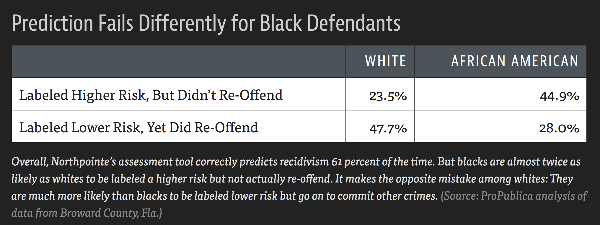
ProPublica Analysis

Shift Gears: Statistical Inference

The ❤️ of statistical inference is quantifying uncertainty
library(tidyverse)
ce <- read_csv("data/fmli.csv")
summarize(ce, meanFINCBTAX = mean(FINCBTAX))
# A tibble: 1 × 1
  meanFINCBTAX
         <dbl>
1       62480.

The ❤️ of statistical inference is quantifying uncertainty

library(tidyverse)
ce <- read_csv("data/fmli.csv")
summarize(ce, meanFINCBTAX = mean(FINCBTAX))
# A tibble: 1 × 1
  meanFINCBTAX
         <dbl>
1       62480.

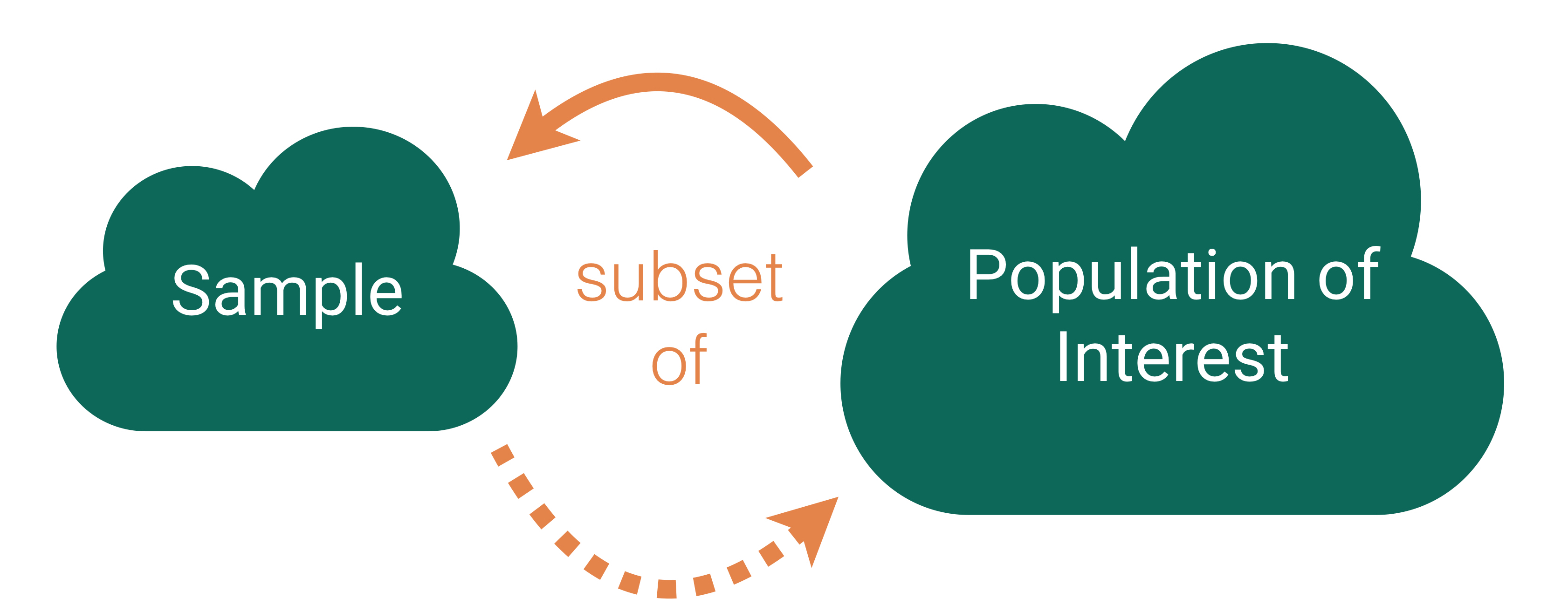
Like with regression, need to distinguish between the population and the sample

  • Parameters:
    • Based on the population
    • Unknown then if don’t have data on the whole population
    • EX: \(\beta_o\) and \(\beta_1\)
    • EX: \(\mu\) = population mean
  • Statistics:
    • Based on the sample data
    • Known
    • Usually estimate a population parameter
    • EX: \(\hat{\beta}_o\) and \(\hat{\beta}_1\)
    • EX: \(\bar{x}\) = sample mean

Quantifying Our Uncertainty

R has been giving us uncertainty estimates:
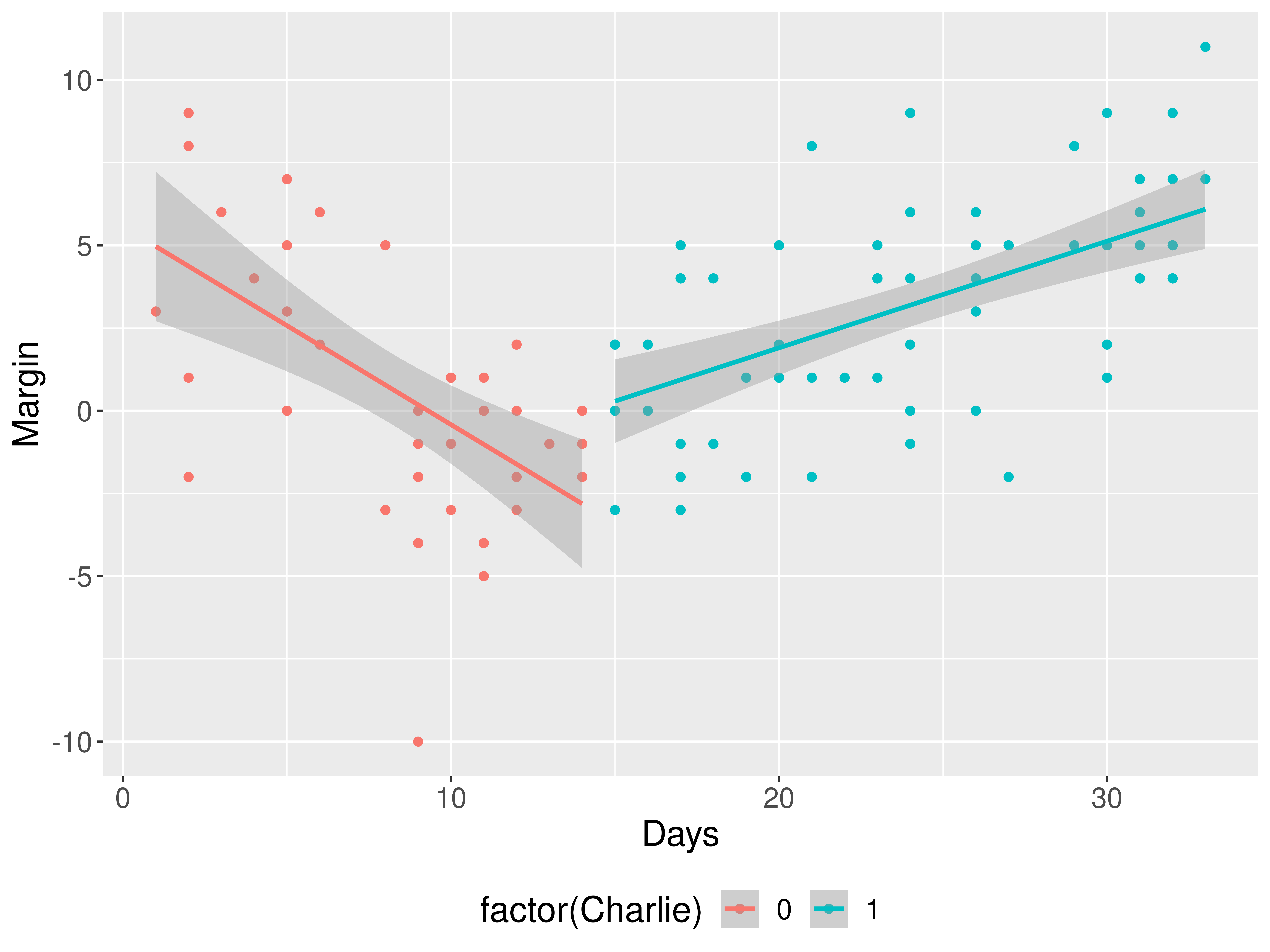
library(Stat2Data)
data("Pollster08")

ggplot(Pollster08, aes(x = Days,
                       y = Margin, 
                       color = factor(Charlie))) +
  geom_point() +
  stat_smooth(method = "lm", se = TRUE) +
  theme(legend.position = "bottom")

Quantifying Our Uncertainty

R has been giving us uncertainty estimates:

library(Stat2Data)
data("Pollster08")
modPoll <- lm(Margin ~ Days*factor(Charlie), data = Pollster08)
library(moderndive)
get_regression_table(modPoll)
# A tibble: 4 × 7
  term                  estimate std_error statistic p_value lower_ci upper_ci
  <chr>                    <dbl>     <dbl>     <dbl>   <dbl>    <dbl>    <dbl>
1 intercept                5.57      1.09       5.11       0    3.40     7.73 
2 Days                    -0.598     0.121     -4.96       0   -0.838   -0.359
3 factor(Charlie): 1     -10.1       1.92      -5.25       0  -13.9     -6.29 
4 Days:factor(Charlie)1    0.921     0.136      6.75       0    0.65     1.19 

Quantifying Our Uncertainty

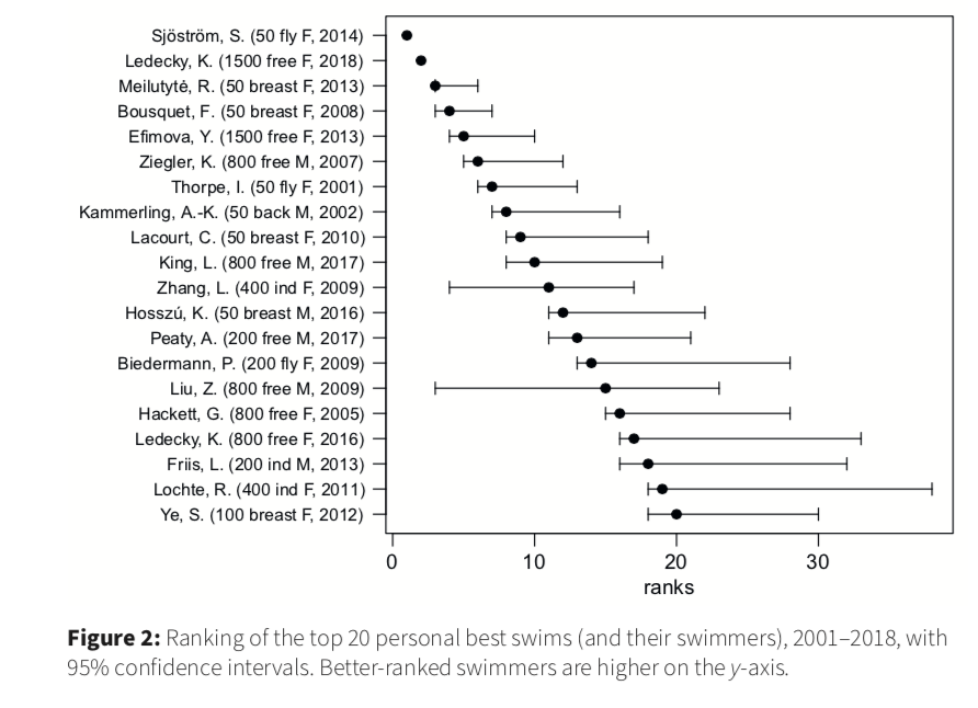
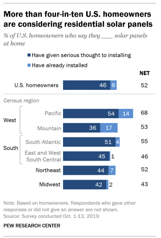
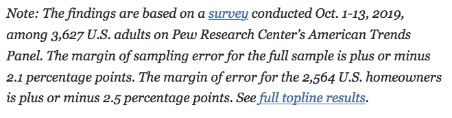
The news and journal articles are also giving us uncertainty estimates:
Quantifying Our Uncertainty

The news and journal articles are also giving us uncertainty estimates:
Statistical Inference

Goal: Draw conclusions about the population based on the sample.

Main Flavors

  • Estimating numerical quantities (parameters).

  • Testing conjectures.

Estimation

Goal: Estimate a (population) parameter.

Best guess?

  • The corresponding (sample) statistic

Example: Are GIFs just another way for people to share videos of their pets?

via GIPHY

Want to estimate the proportion of GIFs that feature animals.

Estimation

Key Question: How accurate is the statistic as an estimate of the parameter?

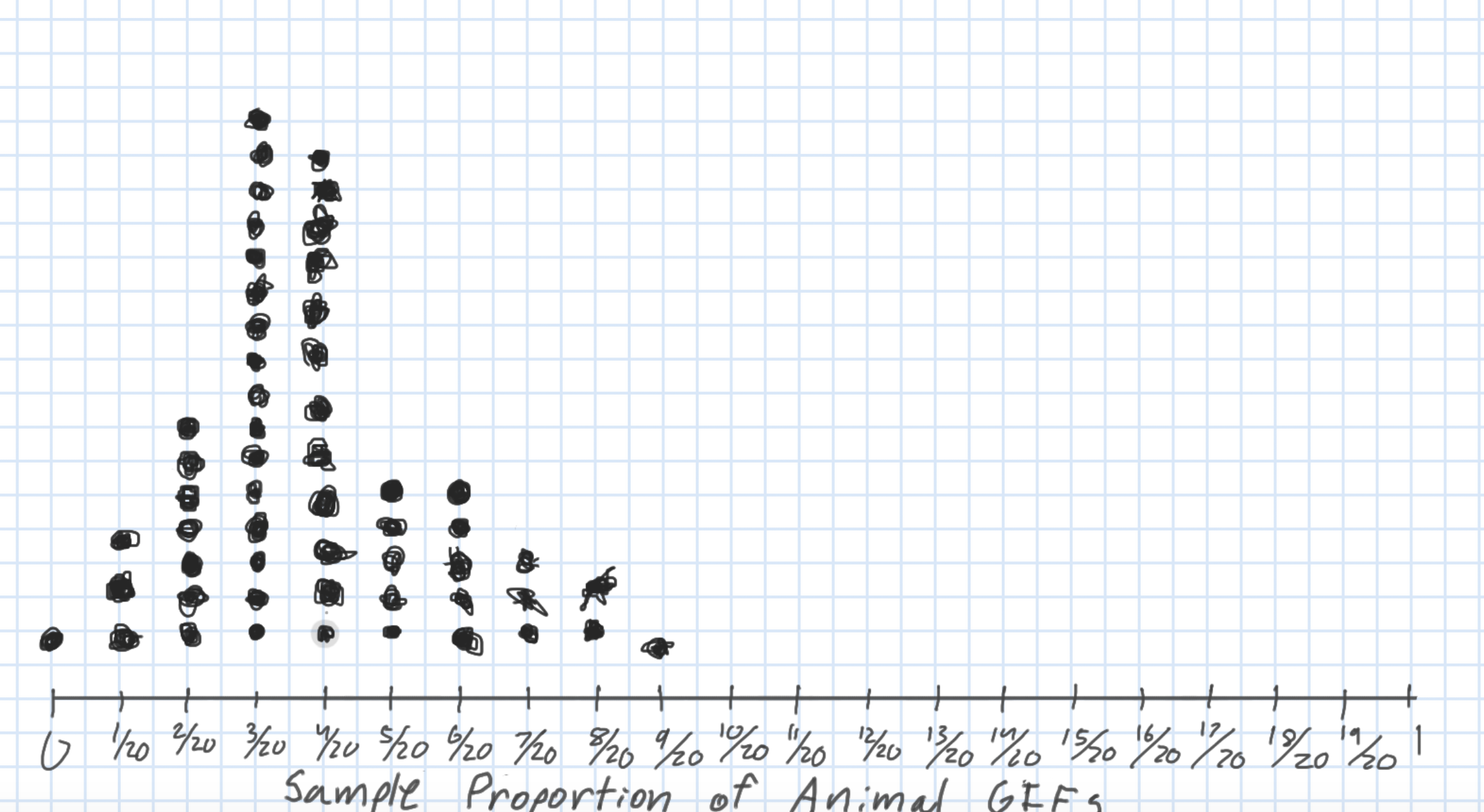
Helpful Sub-Question: If we take many samples, how much would the statistic vary from sample to sample?

Need two new concepts:

  • The sampling variability of a statistic

  • The sampling distribution of a statistic

Let’s learn about these ideas through an activity! Go to bit.ly/stat100gif.

Sampling Distribution of a Statistic

Steps to Construct an (Approximate) Sampling Distribution:

  1. Decide on a sample size, \(n\).

  2. Randomly select a sample of size \(n\) from the population.

  3. Compute the sample statistic.

  4. Put the sample back in.

  5. Repeat Steps 2 - 4 many (1000+) times.

Sampling Distribution of a Statistic

  • Center? Shape?

  • Spread?

    • Standard error = standard deviation of the statistic
  • What happens to the center/spread/shape as we increase the sample size?

  • What happens to the center/spread/shape if the true parameter changes?

Let’s Construct Some Sampling Distributions using R!

Important Notes

  • To construct a sampling distribution for a statistic, we need access to the entire population so that we can take repeated samples from the population.

    • Population = Harvard trees
  • But if we have access to the entire population, then we know the value of the population parameter.

    • Can compute the exact mean diameter of trees in our population.
  • The sampling distribution is needed in the exact scenario where we can’t compute it: the scenario where we only have a single sample.

  • We will learn how to estimate the sampling distribution soon.

  • Today, we have the entire population and are constructing sampling distributions anyway to study their properties!

New R Package: infer


library(infer)
  • Will use infer to conduct statistical inference.

Our Population Parameter

Create data frame of Harvard trees:

library(tidyverse)
library(bosTrees)
harTrees <- camTrees %>%
  filter(Ownership == "Harvard", SiteType == "Tree") %>%
  drop_na(SpeciesShort)

Add variable of interest:

harTrees <- harTrees %>%
  mutate(tree_of_interest = case_when(
    SpeciesShort == "Maple" ~ "yes",
    SpeciesShort != "Maple" ~ "no"
  ))
count(harTrees, tree_of_interest)
# A tibble: 2 × 2
  tree_of_interest     n
  <chr>            <int>
1 no                2707
2 yes                434

Population Parameter

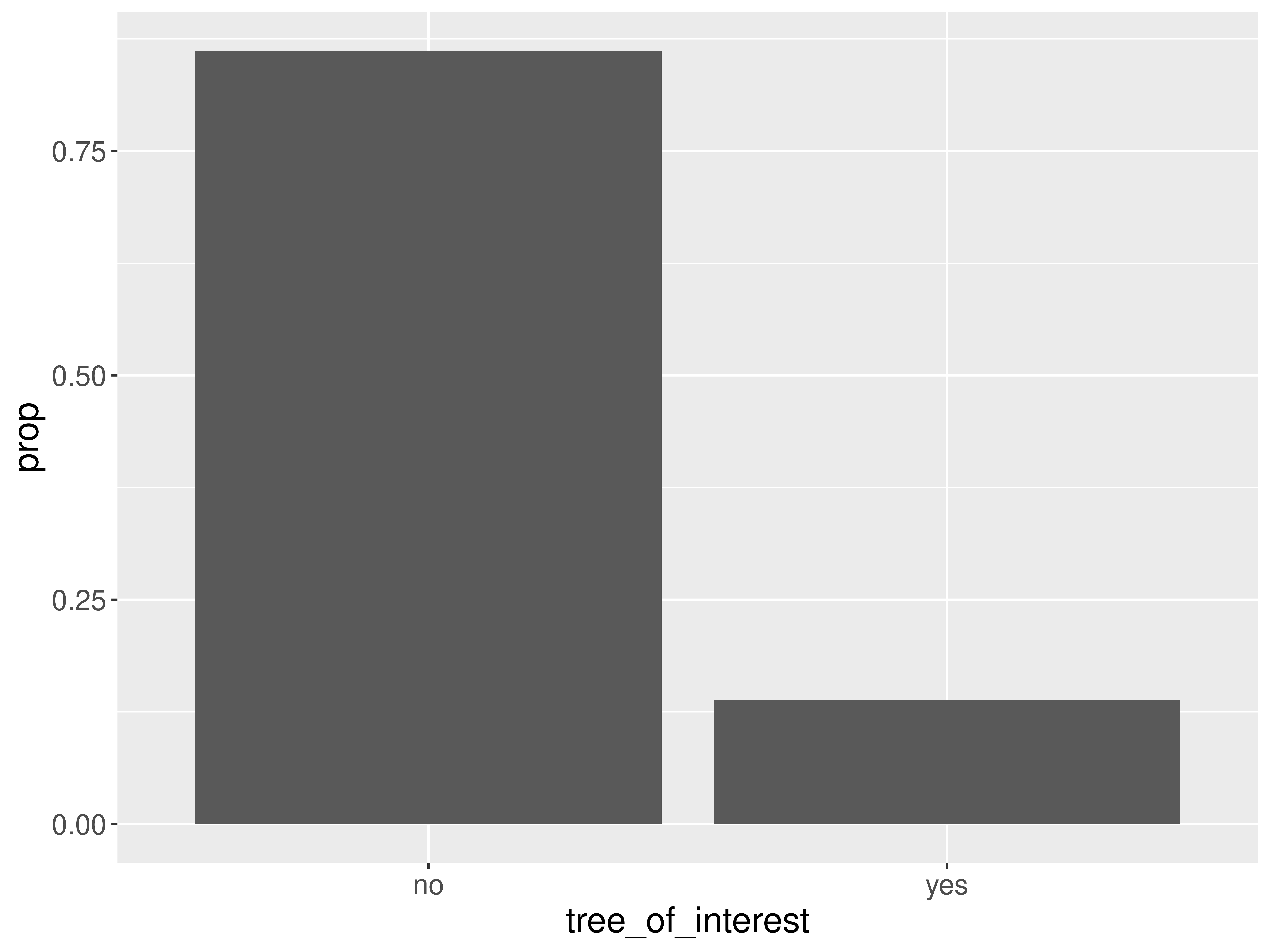
# Population distribution
ggplot(data = harTrees, 
       mapping = aes(x = tree_of_interest)) +
  geom_bar(aes(y = ..prop.., group = 1),
           stat = "count") 

# True population parameter
summarize(harTrees, 
          parameter = mean(tree_of_interest == "yes"))
# A tibble: 1 × 1
  parameter
      <dbl>
1     0.138

Random Samples

Let’s look at 4 random samples.
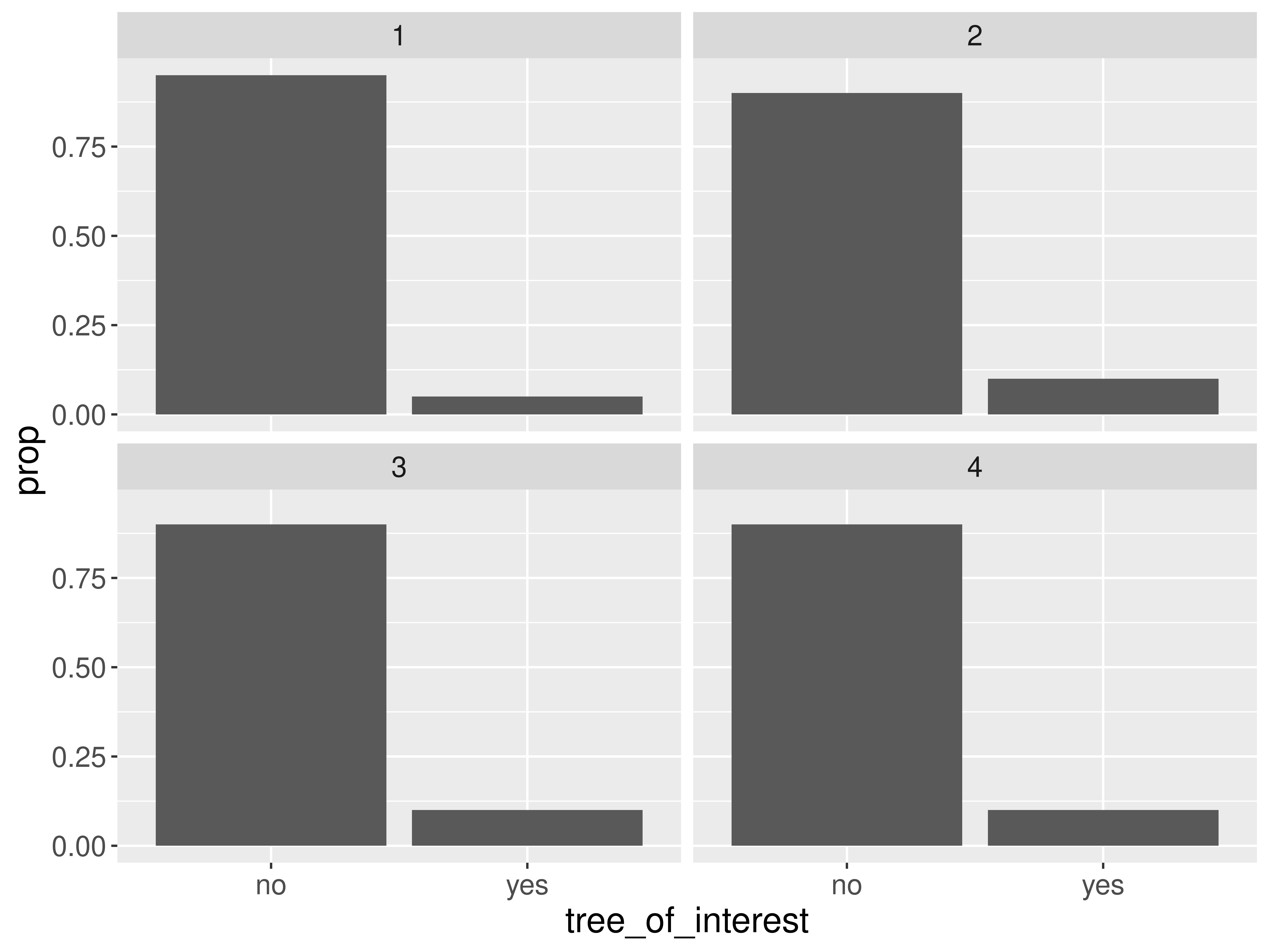
# Draw random samples
samples <- harTrees %>% 
  rep_sample_n(size = 20, reps = 4)
  
# Graph the samples
ggplot(data = samples, 
       mapping = aes(x = tree_of_interest)) +
  geom_bar(aes(y = ..prop.., group = 1),
           stat = "count") +
  facet_wrap( ~ replicate)

Constructing the Sampling Distribution

Now, let’s take 1000 random samples.

# Construct the sampling distribution
samp_dist <- harTrees %>% 
  rep_sample_n(size = 20, reps = 1000) %>%
  group_by(replicate) %>%
  summarize(statistic = 
              mean(tree_of_interest == "yes"))

# Graph the sampling distribution
ggplot(data = samp_dist, 
       mapping = aes(x = statistic)) +
  geom_histogram(bins = 14)
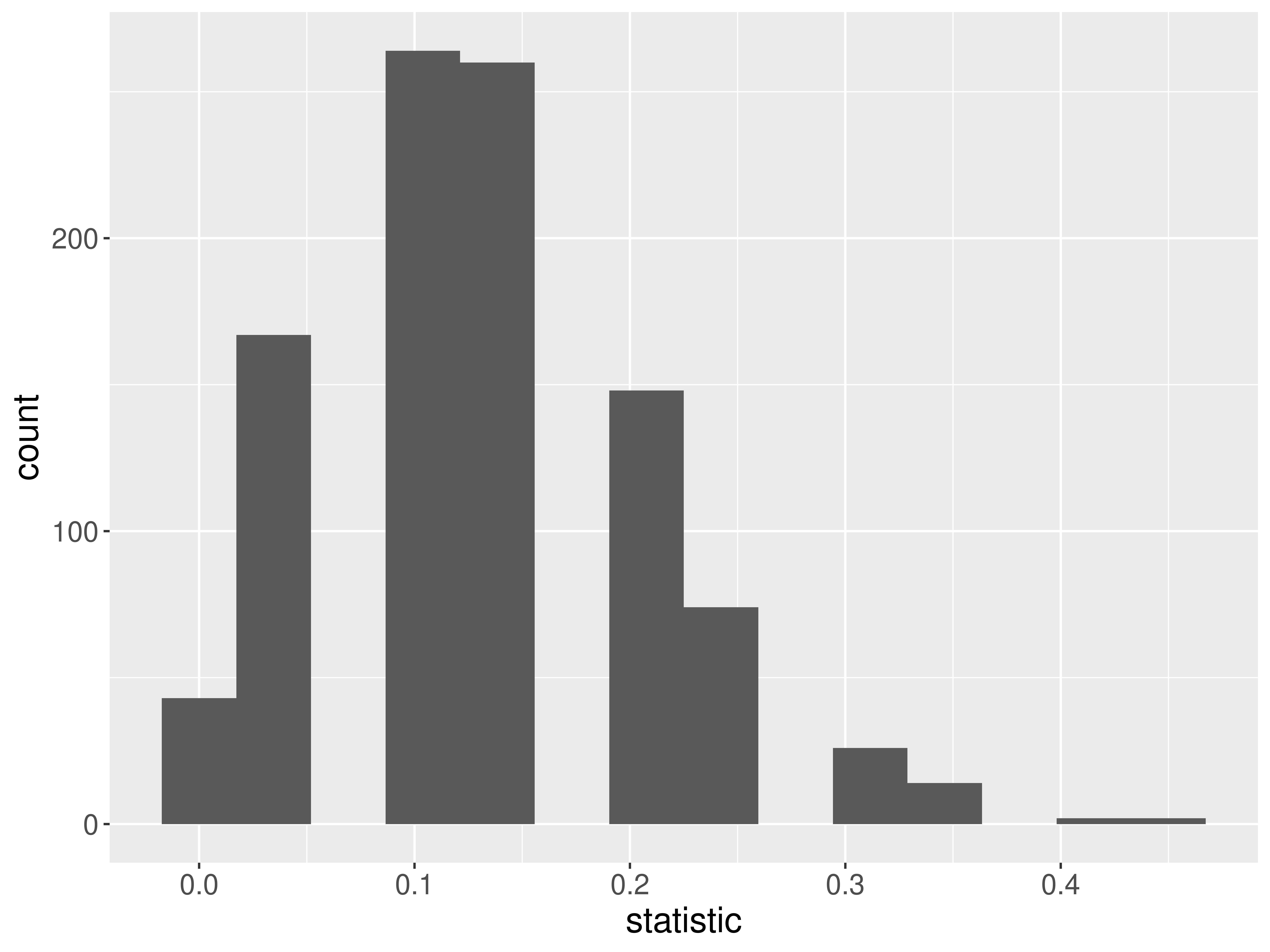
  • Shape?
  • Center?
  • Spread?

Properties of the Sampling Distribution
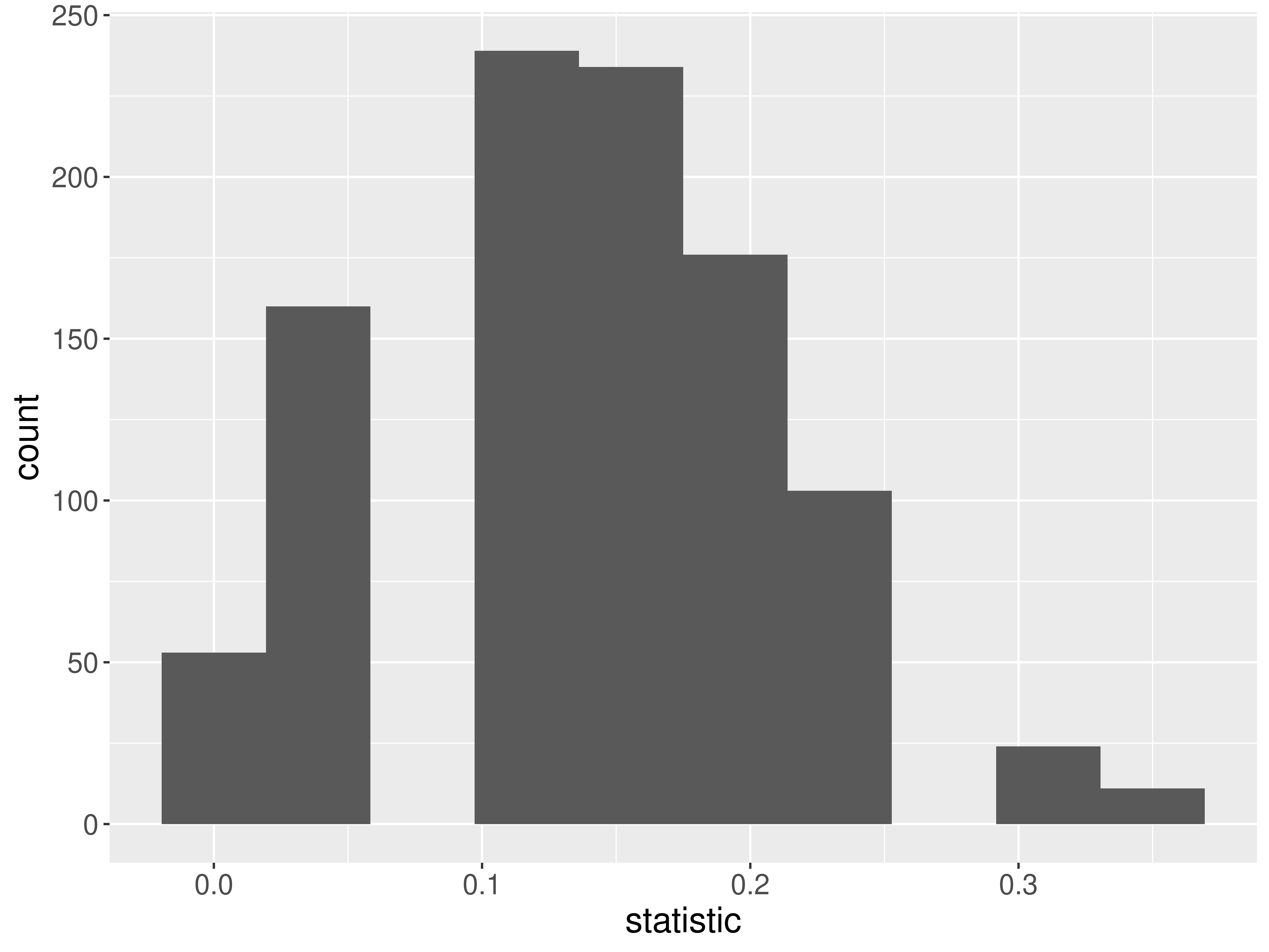
summarize(samp_dist, mean(statistic))
# A tibble: 1 × 1
  `mean(statistic)`
              <dbl>
1             0.139
summarize(samp_dist, sd(statistic))
# A tibble: 1 × 1
  `sd(statistic)`
            <dbl>
1          0.0757

The standard deviation of a sample statistic is called the standard error.

What happens to the sampling distribution if we change the sample size from 20 to 100?

# Construct the sampling distribution
samp_dist <- harTrees %>% 
  rep_sample_n(size = 100, reps = 1000) %>%
  group_by(replicate) %>%
  summarize(statistic = 
              mean(tree_of_interest == "yes"))

# Graph the sampling distribution
ggplot(data = samp_dist, 
       mapping = aes(x = statistic)) +
  geom_histogram(bins = 20)
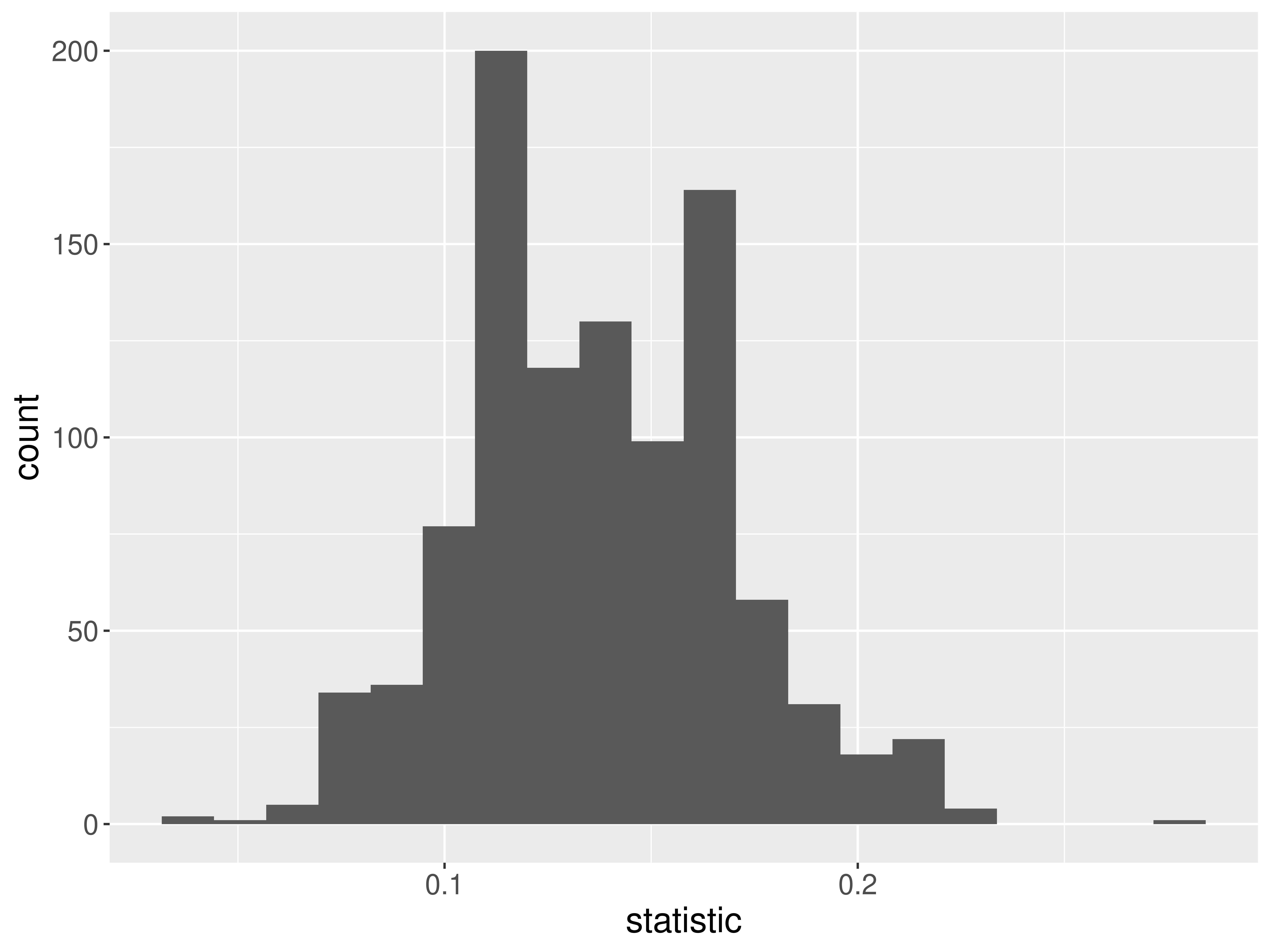
summarize(samp_dist, mean(statistic), 
          sd(statistic))
# A tibble: 1 × 2
  `mean(statistic)` `sd(statistic)`
              <dbl>           <dbl>
1             0.138          0.0326

What if we change the true parameter value?
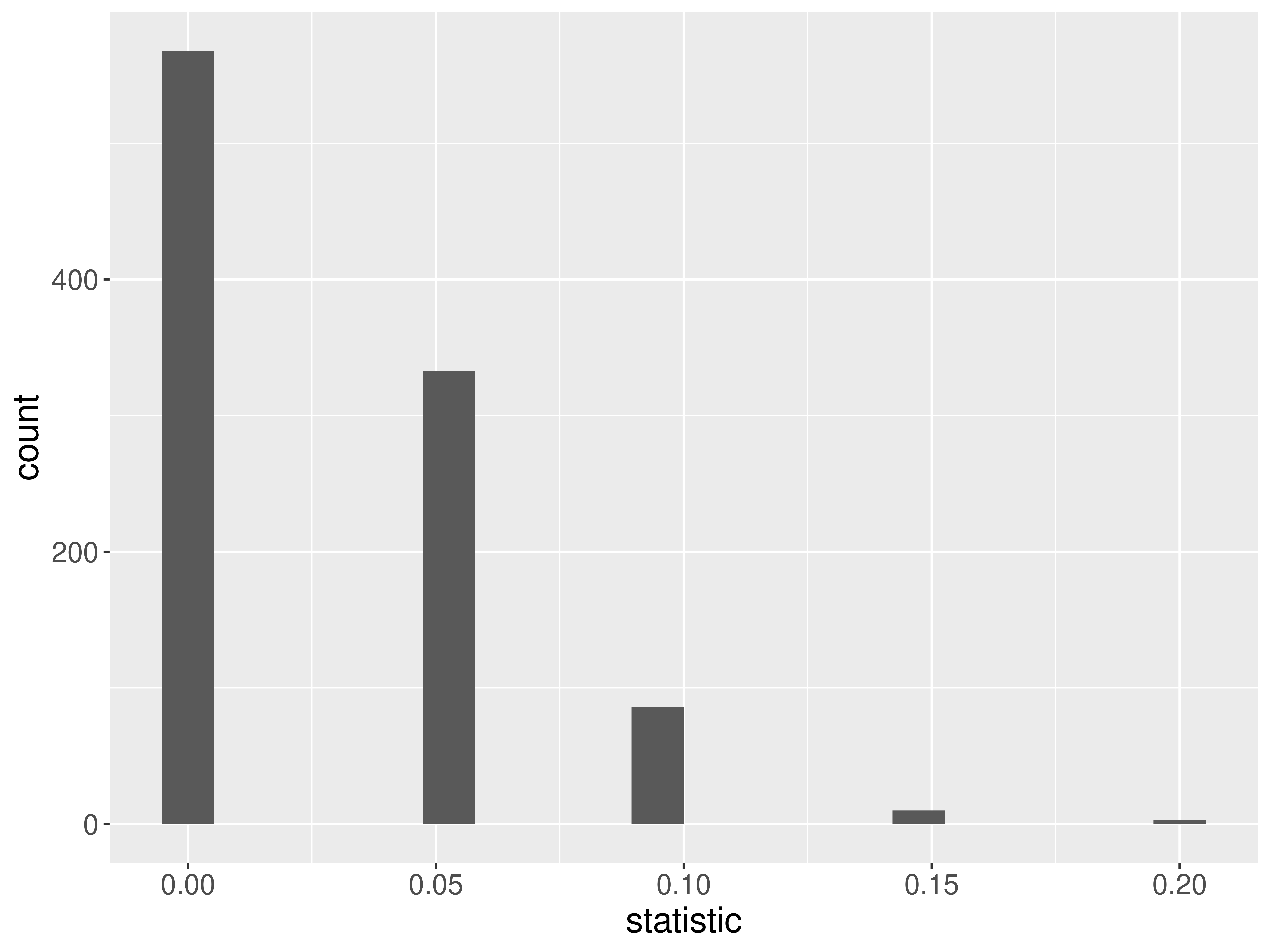
# Construct the sampling distribution
samp_dist <- harTrees %>%
  rep_sample_n(size = 20, reps = 1000) %>%
  group_by(replicate) %>%
  summarize(statistic =
              mean(SpeciesShort == "Cherry"))

# Graph the sampling distribution
ggplot(data = samp_dist,
       mapping = aes(x = statistic)) +
    geom_histogram(bins = 20)

summarize(samp_dist, mean(statistic),
          sd(statistic))
# A tibble: 1 × 2
  `mean(statistic)` `sd(statistic)`
              <dbl>           <dbl>
1            0.0274          0.0359

On P-Set 6:

Will investigate what happens when we change the parameter of interest to a mean or a correlation coefficient!

Key Features of a Sampling Distribution

What did we learn about sampling distributions?

  • Centered around the true population parameter.

  • As the sample size increases, the standard error (SE) of the statistic decreases.

  • As the sample size increases, the shape of the sampling distribution becomes more bell-shaped and symmetric.

  • Question: How do sampling distributions help us quantify uncertainty?

Cliffhanger:

If I am estimating a parameter in a real example, why won’t I be able to construct the sampling distribution??